Meteorological considerations in WindTrax
This section of WindTrax help will introduce the basic meteorology underlying the models used in WindTrax.
Micrometeorology
To understand processes involving transport by the wind, we need some understanding of the wind itself. Micrometeorology is the science of the lower, turbulent region of the atmosphere (the "Planetary Boundary Layer," or PBL for short), and it focuses on the wind, the temperature, the humidity, and the processes that control them. The "Atmospheric Surface Layer" (hereafter ASL) is a sub-layer of the PBL. For our purposes, the ASL is the lowest 50 to 100 meters of the atmosphere, within which occur the environmental processes that have generated your interest in WindTrax.
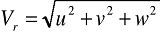
The wind is air in motion. One cannot speak of motion without reference to a coordinate system: ours will be the familiar rectangular coordinates (x, y, z), where the z-axis is the local vertical. Relative to this reference, the wind at any point is characterized by a strength (Vr) and two directions (the azimuth angle, which we refer to as wind direction; and the elevation angle, which is seldom measured). Equivalently, we may say the wind has three "components," usually called (u, v, w), which are the wind velocities along each of the three axes x, y, z. In a common notation, the wind vector (u, v, w) is represented by the shorthand u (note the use of bold to denote a vector). Thus u is the wind-velocity along the x direction, etc; and the wind speed Vr is the resultant of these three velocities, given by the formula
In micrometeorology and many applied sciences, we often measure the wind using "cup anemometers." These sense the "cup windspeed" (s) which is just the resultant
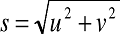
of the two horizontal components.
What controls the wind? In a word, forces. One among these merits special: the buoyancy force exerts a crucial control over the vertical wind and turbulence, and so modulates vertical mixing of air properties. This implies that the motion of the air (wind) is not independent of the other attributes of the air, most specifically temperature and humidity. Today's scientific "model" of the wind unites a set of causally inter-coupled variables: the wind, the temperature, and the humidity.
Now we have to grapple with the level of detail with which our science and our models describe "the wind."
Focus on Statistics (Averages and Standard Deviations)The Critical Importance of Symmetry ("Horizontal Uniformity")>
Monin-Obukhov Similarity Theory (MOST) for the Profiles in the ASL
Wind transport
Focus on Wind Paths
What are "Fluxes"?
The Q Inference problem
Key LS Model Variables
Back to Table of Contents
Focus on Statistics (Averages and Standard Deviations)
It is likely familiar to you that atmospheric variables observed near the ground are turbulent, meaning that they fluctuate unpredictably in time and space. Let us take for example the temperature, whose symbol will be T. Let us acknowledge that T is a field (i.e. it varies in space and time). Symbolically, we indicate this by writing T = T(x, y, z, t). It goes without saying that the other atmospheric variables are also fields; cup windspeed s = s(x, y, z, t), and so forth.
It is not possible to predict the chaotic field T = T(x, y, z, t) in all its overwhelming complexity throughout the atmospheric continuum; realistically, we must instead focus on the statistics of T. Micrometeorological statistics are defined over an interval of time long enough to "see" the whole act that turbulence puts on for us, but not so long that "external" factors like the rising or setting of the sun sneak in to steal our attention. In practice, the averaging interval is usually between 15 and 60 minutes.
The first and foremost statistic of T is its average value, denoted T . The next most important statistic is the standard deviation (σT). The standard deviation is also known as the "root-mean-square deviation," and it quantifies the fluctuations of T about its average T . If you are somewhat familiar with statistics you know the standard deviation measures the "spread" of a probability distribution about its average.
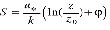
The horizontal wind field is effectively described (perhaps summarized is a better word) in terms of the average cup windspeed S, defined by the equation
(the average value of the square-root of the sum of the squares of u and v), and the average wind direction α . The same information is alternatively provided by the two average horizontal velocity components U and V. If we need more statistical detail on the wind, we refer to (and build theories for) the standard deviations σu, σv, σw. Only very rarely is there any benefit to climbing to an even higher level of statistical detail in describing the wind (e.g., skewness and kurtosis).
There are other important micrometeorological statistics; let us mention only the "covariance" wT (the average value of the product of T with the vertical velocity w measured at the same point). wT is closely related to the average vertical heat flux QH crossing through the atmosphere. But for now, the next point is to ask, to what extent do our averages and other statistics themselves vary in time and space?
The Critical Importance of Symmetry ("Horizontal Uniformity")Back to micrometeorology
The Critical Importance of Symmetry ("Horizontal Uniformity")
The statistics of the atmosphere themselves vary in time and space. For example, the time-average temperature T = T (x, y, z, t), where now the variation in time t will be "slower" due to our having averaged (we shall have "smoothed out" most of the turbulent fluctuations; but there will remain the slow diurnal cycle; and an even slower variation as the air-masses come and go. Let us neglect these slow variations in time, and write T = T (x, y, z, t), it being understood that T may be different for each subsequent 30 minutes (or so).
Supposing that the ground surface is quite uniform in its properties, such as for a prairie; is it reasonable to expect that in the ASL the wind will be in equilibrium with this monotonous surface, and therefore that its average properties (ie. statistics) might be invariant in the horizontal plane? This, at least, is the customary assumption in micrometeorology. Wherever the assumption is valid, we may (for example) say, "the average windspeed S no longer varies with x, y, z, t - only with z." Symbolically, we convey this by writing S= S(z), and so on.
Whenever and wherever this simplification (i.e. assumed horizontal homogeneity) is valid, we can give a compact description of the state of the ASL in terms of the vertical profiles of S(z), T , average humidity H , and so forth. Mathematical formulae for these profiles have been found, by a combination of measurements (mostly over prairies) and dimensional analysis (called Monin-Obukhov Similarity Theory). These formulae are at the heart of WindTrax, and thus restrict its applicability to surfaces that are reasonably uniform. We should also mention that pathological ASL's, such as during heavy fog, or in the middle of a thunderstorm, are not described by WindTrax.
Monin-Obukhov Similarity Theory (MOST) for the Profiles in the ASLBack to micrometeorology
Monin-Obukhov Similarity Theory (MOST) for the Profiles in the ASL
Monin-Obukhov Similarity Theory (MOST) posits that if the ASL is horizontally-uniform, then the statistical properties of the wind (e.g. S(z)) are governed by Ground-air friction, or drag. This factor is characterized by two "scales": an attribute of the ground itself, the ground roughness length Zo; and a measurable attribute of the windflow called the "friction velocity" u*.
In a simple dichotomy, the influence of buoyancy can be reduced to a distinction between day and night. We assume "day" means sunny and "hot ground under colder air," while night means "cold ground under warmer air." Daytime conditions normally imply "instability" or "unstable stratification", and night-time conditions normally imply "stable stratification." Why the link between temperature stratification and stability? Because if cool air is overlain by warm air, vertical motion is suppressed (and vice versa). Thus the "stratification" of the air has an enormous influence on the properties of the ASL. Deepening the level of detail, there is a third stability category, namely "neutral stratification". In neutral stratification heat is uniformly mixed, as when it is windy or when the sky is heavily clouded. But in speaking of categories, we speak qualitatively. Actually, there is a continuum of states. This continuum is characterized by the Obukhov length L, which we specify in meters: L is negative (positive) in unstable (stable) stratification. The larger its magnitude (absolute value), the smaller are buoyancy forces; neutral stratification is represented by 1/L = 0, ie. L is infinitely positive, or infinitely negative.
If we are speaking of a suitably uniform site, then all properties of the ASL that we need to resolve are known - at least the moment we can specify the three ASL scales u*, Zo, and L. As an example, the vertical profile (vertical structure) for the standard deviation of the vertical velocity, can be written symbolically as
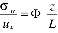
This equation says, "the friction velocity u* is the scale for the standard deviation of w, and L is the scale for height z; provided it is made dimensionless on (scaled on) its proper scale, w is a function only of the height made dimensionless on the height scale." Field experiments have determined the form of the function. In the limit of neutral stratification (as L becomes infinitely large), σw / u* = constant = 1.3.
Measuring or estimating ZoMeasuring L directly
Estimating L from a Richardson number
Measuring L and Zo from S and T profiles
Estimating L from the standard deviation of wind direction
Back to micrometeorology
Measuring or estimating Zo
The logarithmic wind law for neutral stability defines the roughness length Zo. It is the height at which where the extrapolated windspeed S = 0. Zo depends on the aerodynamic roughness of the surface. It is related to the height of the surface roughness elements.
If a set of S observations (taken during neutral stability) is plotted on a semi-log graph, then Zo is given by linearly extrapolating to the height where S = 0. The value of Zo can also be inferred from S as part of a comprehensive Zo and L fitting algorithm (see Measuring L and Zo from S and T profiles).
An alternative to Zo measurement is selecting a value from a literature report on the specific surface type of interest. The use of these literature values of Zo is the option we suggest for most users. In WindTrax, several common surface types and typical Zo values have been tabulated. Clicking on the map surface and selecting a surface type (see selecting Zo) provides access to these values.
Back to Monin-Obukhov Similarity TheoryMeasuring L directly
The stability length L can be calculated directly frommeasurements of a 3-D sonic anemometer (with an integrated fine-wire thermocouple for calculating heat flux). A sonic anemometer can give the friction velocity u* and the sensible heat flux wT . The value of L is
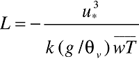
where k is the von Karmen constant (0.4), g is gravitational acceleration, and Tv is the virtual temperature in degrees K (there is little error in assuming Tv = T).
Back to Monin-Obukhov Similarity TheoryEstimating L from a Richardson number
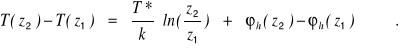
Another method of inferring L is to assess the Richardson number Ri, which is a measure of atmospheric stratification. Ri is calculated from differences in average temperature T and windspeed S between two heights z2 and z1. It is often approximated as
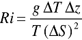
where g is gravitational acceleration, and T is given in degrees K. The value of L and Ri are related. A common assumption is that
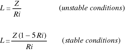
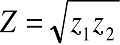
where Z is taken as the measurement height for Ri. We suggest using
 .
.
Estimating L and Zo from S and T Profiles
The Obukhov length L and the roughness length Zo can be estimated simultaneously from a vertical profile of windspeed S. Increased accuracy can be achieved if average temperature profiles (T) are also available. The measured S and T profiles are fit to theoretical curves which are known to describe S and T in the atmosphere. These theoretical curves are functions of height z, Zo, L, and the friction velocity u*.
The theoretical windspeed profile that describes how the average windspeed changes with height is
where k is von Karman's constant ( 0.4), and is a stability correction term. For example, Businger et al. (1971) and Paulson (1970) give
where
 .
.
A similar functional form exists for the temperature profile:
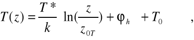
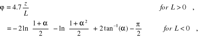
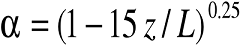
where T* is a temperature scale, z0T is a temperature roughness length (~ Zo), and T0 is a surface temperature. This profile actually describes the virtual potential temperature, not actual temperature, but this slight error has been ignored. A stability correction h is given in Garratt (1992):
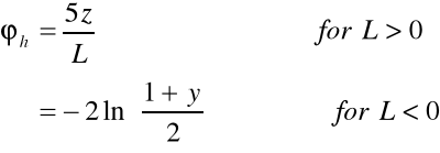
where y = (1 - 16z/L)0.5. The T profile equation contains the parameters z0T and T0 which are not needed in WindTrax, and it is more useful to write a temperature difference between two heights z1 and z2 as
Using the above combination equations it is possible to find a best fit value of Zo and L (and u*) for a given measured profile of S and T.
Back to Monin-Obukhov Similarity TheoryEstimating L from the Standard Deviation of Wind Direction
A potentially practical way to estimate L is by examiningthe standard deviation of the wind direction during a measurement period (e.g. over 30 minutes). The method is based on the fact that during unstable conditions the wind direction is more variable than during stable cases. Of the methods for finding L, this is the simplest and cheapest. Because WindTrax requires a wind vane to record average wind direction already, there is no additional instrumentation required to give . Unfortunately the method is not as accurate as the previously discussed techniques for determining L, and we are hesitant to recommend it.
We can closely approximate the as σv/S, where σv is the standard deviation of the lateral wind velocity v. We can take MOST estimates of both σv and S to calculate a theoretical corresponding to Zo, L, and a measurement height z. Since we know Zo and z, fitting the theoretical curve to the measured gives us an estimate of L.
This technique for finding L is prone to error. During times where the average wind direction is slowly changing (which is often), is increased over that predicted by MOST. This is not so bad during unstable conditions, but it can lead to serious errors in stable cases. This situation can cause a mistaken classification of a stable period into unstable. We have two suggestions to minimize error. The first is to reduce the measurement interval. We suggest 30 minutes or less (10 minutes would be ideal). As well we suggest the user supply a day-night indicator to WindTrax. There is then an option of WindTrax to not allow a nighttime situation to be classified as unstable.
Back to Monin-Obukhov Similarity TheoryWind Transport
If you stand downwind of a lawn sprinkler the wind blows spray in your face, except during the lulls; wind transport is about that simple. If we "know" the wind, there is no reason to be surprised by the path of the spray. The only complication is that the wind is turbulent, so spray particles do not travel in straight lines.
Because of this complication it is customary (though strictly wrong) to think of turbulent wind transport as a "diffusion" (or mixing) process. By far the majority of wind transport algorithms treat turbulent transport as "turbulent diffusion." They ascribe to the atmosphere an effective "eddy diffusivity" (K). This can be made to work, but it is fundamentally wrong.
WindTrax takes a more natural approach to calculating wind transport. It uses the Lagrangian stochastic (LS) method of calculating wind paths. From these wind paths it is possible to predict the "flux" of water from the sprinkler to your face: given the total amount of water coming from the sprinkler and the wind conditions.
The problem of the lawn sprinkler could also be reversed. Instead of calculating the amount of spray blowing in your face (given the total amount of water coming from the sprinkler), can we calculate the total amount of water exiting the sprinkler given the amount of water hitting my face? We call this the Q inference problem, and it is a problem WindTrax was designed to solve.
Focus on Wind PathsBack to micrometeorology
Focus on Wind Paths
WindTrax treats turbulent transport exactly for what it is & WindTrax mimics a particle's motion in a re-constructed random wind field u = u(x,y,z,t). The key is that this random wind field has precisely the right statistical patterns for the specified atmosphere and terrain; the right profiles in the three components of average velocity U(z), V(z), W(z); and the right profiles of the velocity standard deviations σu, σv, σw, and so on. The heart of WindTrax is its Lagrangian Stochastic (LS) particle trajectory model; here "Lagrangian" is a technical adjective meaning "particle-following", and "stochastic" is a fancy word for "random."
One of the wonderful attributes of an LS model is that one can "run the film backwards." One may calculate trajectories forwards in time, from a source to a destination/receptor; but one may equally well spot a particle at a detector, and ask, "Oh, where might this have come from?" Indeed one can do better than ask the question - one may answer it (probabilistically, which is all that is necessary). This flexibility makes WindTrax a powerful package for the analysis of environmental problems that crucially involve wind transport.
For technical details on the LS model for wind transport, please see:
Wilson, J.D., and B.L. Sawford, 1996: Lagrangian stochastic models for trajectories in the turbulent atmosphere. Boundary Layer Meteorology 78:191-210.
Flesch, T.K., J.D. Wilson, and E. Yee. 1995. Backward-time Lagrangian stochastic dispersion models, and their application to estimate gaseous emissions. Journal of Applied Meteorology. 34:1320-1332.
What are fluxes?Back to micrometeorology
What are "Fluxes"?
When you stand downwind of the sprinkler your face gets wet. But how wet? That depends on how much water you intercept. And how much water you intercept depends on your rate of interception ofwater - the "flux" of water. That in turn depends on your bodily surface area, on the loading of spray in the airstream, and on the velocity of the airstream: no spray & no interception & no air motion = no flux.
The quantity of some entity suspended in air is usually specified in terms of a mass density, say c (kg / cubic meter). Air motion, of course, is indicated by a velocity vector u. The "mass flux density" is just the product q = u c (kg / square meter / sec). The vector flux q is the natural measure of the rate of transport of the component whose concentration is c, and has three components, q=(qx, qy, qz), where qz = w c is the vertical flux (etc). Very often in the environmental problems the aim is to determine the average value of the vertical flux
from a source, whether that be ammonia from a feedlot, or methane from a landfill. What is wanted is the value of this flux at the air-ground interface, ie. the emission rate Qz(x, y, z = 0). Many of the alternative techniques for flux-determination require a condition of symmetry (sufficient fetch of source) to justify an assumption that is independent of x, y and z.
The Q Inference problemBack to micrometeorology
The Q Inference problem
Let us consider a hypothetical use of WindTrax: to quantify the emission rate Q (kg / square meter / s) of ammonia from a small plot of treated bare soil, surrounded by untreated soil. Assume the surface is otherwise homogeneous. If the goal is a measurement technique that does not disturb the soil and airflow, your only option is some type of micrometeorological technique in which you measure the ammonia added to the air in passing over the plot. But a formidable obstacle is that the size and shape of our plot are arbitrary& and so lets us say that the plot may be so small as to render inapplicable the standard micrometeorological methods (e.g. eddy covariance, flux gradient techniques).
The quickest way to introduce you to solution of this problem using WindTrax (in conjunction with the simplest and most economical of field measurements) is to point out that it is a dimensionally correct statement that
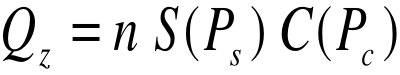
where n is an unknown dimensionless number, S(Ps) is the average cup windspeed measured nearby at an (arbitrary) point Ps, and C(Pc) is the time-average gas concentration measured at another arbitrary point Pc downwind from source plot. What this implies is that if you knew the numeric value of n, then all you need do is measure S(Ps) and C(Pc), and the formula would give you what you want, Qz! By the way, Pc and Ps could be the same point; this is a matter of convenience.
Back to micrometeorologyKey LS Model Variables
For most users the internal details of the LS dispersion model are not important. We have tried to keep most of the intricacies hidden. However, there are two key variables that the user should be aware of, and may need to change.
The most important detail is the number of "particles" used in the LS model simulations (N). Typically N = 10,000 to 50,000 particles. In any given situation, the larger the value of N, the lower the model uncertainty. When the source region decreases in size, or when the concentration sensor becomes more distant from the source, a larger N is often required (see selecting N). It may also be necessary to increase N if the concentration sensor is located near the edge of the tracer plume emanating from the source. There is larger uncertainties in the LS model predictions near the plume edge (i.e. fewer model particles occur at the edge of the plume). In some cases increasing N does not decrease the model uncertainty. If the concentration sensor is outside the source area, and the wind direction is away from the sensor, no prediction of Q is possible. Increasing N has no effect.
The other important LS variable is particle-tracking distance. When WindTrax calculates a touchdown catalog it tracks particles for a distance X upwind. X must be larger than the furthest point the source is away from the sensor where C is observed or predicted. WindTrax automatically calculates X for a given problem. The selection of X is not just determined by the problem at hand. The greater the value of X the greater the utility of a catalog: a catalog with a large X will be useful for many problems, while one with a small X has limited potential. The user may therefore select a larger value of X than needed for a problem in order to increase the usefulness of that catalog (see selecting tracking distance).
The tracking distance X should generally not exceed 1000 m. This means WindTrax should not be used for problems where the source-sensor scale is greater than 1000 m. The reason lies in the accuracy of the LS model. The LS model in WindTrax is valid for the ASL, which is the lowest 50-100 m of the atmosphere. To track tracers beyond 1000 m in principle requires model accuracy above a height of 50 m: material transported beyond 1000 m may have been transported above 50 m. The argument is that if WindTrax does not accurately simulate transport above 50 m, it cannot make accurate predictions beyond 1000 m. We believe the 1000-m maximum scale is conservative.
Back to micrometeorology