An introduction to WindTrax

WindTrax is a graphically-based interface. Using the mouse pointer, you will draw a map of the actual situation you wish to simulate, adding symbols representing sensors for wind and concentration, and coloured shapes to represent area sources. Although they have default values, the properties of the objects on the map can be tailored to your experimental set-up by double-clicking on them. When everything is in place, you simply click the Start button (or select Simulation|Start from the main menu) to find the unknown values on the map. That's it!

Two types of problems
Drawing the map
Supplying experimental information
Generating the answer
WindTrax output
LS dispersion models
Sources of error and uncertainty

Back to Table of Contents

---

Two types of problems

WindTrax is used for two basic types of problems. The first is the calculation of average gas concentration (C) downwind of a source, given the emission rate (Q). The second is to determine Q given a C observation downwind of the source (Q inference problem). Both of these problems require knowledge of the "Q-C relationship" (i.e. the ratio C/Q), and this is the function of WindTrax.

Predicting concentration with WindTrax
Inferring Q with WindTrax

Back to WindTrax introduction

---

Predicting concentration with WindTrax

WindTrax can be used to predict the average concentration C downwind of known emission sources. In this case "known" means the areal extent of the source is well-defined, and Q is also known. WindTrax can predict C at one or many locations, and with one emission source or many sources. WindTrax must know the size, shape, and location of the sources; the Q values; the location of the desired C predictions; as well as the meteorological conditions.

WindTrax allows for only quasi-continuous emission sources, and assumes Q is constant during a measurement period (e.g. 30 minutes). WindTrax was designed for terrain with short vegetation (less than 1 meter in height) or no vegetation at all.

Inferring Q with WindTrax

Back to types of problems

---

Inferring Q with WindTrax

WindTrax can be used to infer a source emission rate Q from an observation of average concentration C downwind of the source. This requires knowledge of the "C-Q relationship". WindTrax calculates this relationship (see Q inference problem.

WindTrax must be provided with the size, shape, and location of the source; the location of the observed C; and the meteorological conditions.

WindTrax is for surface sources only. Determining Q from elevated sources is not possible. WindTrax allows for only quasi-continuous emission sources, and assumes Q is constant during a measurement period (e.g. 30 minutes). WindTrax was designed for terrain with short vegetation (less than 1 meter in height) or no vegetation at all.

Back to types of problems

---

Drawing the map

Most applications of WindTrax will be to solve problems with at least one emission source and one concentration sensor. The location of each must be defined. The heart of the WindTrax interface is a surface map on which users draw sources and sensors. When WindTrax is opened a mapping area is displayed. By default, North is up, and the grid lines are spaced 2.0 m apart; these default features can be changed (see Map Grid and Orientation in the User's Guide.)

WindTrax provides a set of drawing tools for sources. Elliptical, rectangular, and irregular area sources can be drawn, rotated, and moved on the map (see Area Sources in the User's Guide). Point sources can also be added to the map (see Point Sources). The Tape Measure tool, magnifying glass, and various displays help in precisely positioning and scaling the map objects.

Two types of known-concentration sensor can be drawn: point concentration sensors measure C at a single point, while line sensors measure C along a straight line. An open-path laser is a line sensor.

Back to WindTrax introduction

---

Supplying experimental information

Four atmospheric variables are crucially important for WindTrax and must be specified by the user. These are:

Average windspeed S. Typically measured every 30 minutes. The location of the S measurement is arbitrary (assuming horizontal homogeneity), and a convenient height is often selected (e.g. 1.5 m above ground). A cup anemometer, prop-vane (combination windspeed and direction sensor), or sonic anemometer can be used to get S. In WindTrax, wind speed is specified by placing a single anemometer on the map.

Average wind direction θ . Typically measured every 30 minutes. Wind direction can be measured at any location using a stand-alone wind vane, a propvane, or sonic anemometer. For the simulations, direction is specified by the same anemometer that is providing the wind speed.

Atmospheric stability. The Obukhov length L quantifies of stability. Typically measured every 30 minutes. On a typical sunny day L is positive (unstable atmosphere), while at night L is usually negative (stable atmosphere). L can be directly measured using 3-D turbulence anemometers, inferred from vertical profiles of S and T, or estimated from the standard deviation of wind direction during a measurement period (see measuring stability). In older versions of WindTrax, a special Stability Sensor, added automatically to the map, allowed the user to specify stability. This method is no longer used in Version 2.0; stabiity is now specified in the Surface Layer Model object.)

The surface roughness length Z_o. For a bare soil, Z_o may be 0.005 m, while over a wheat field it may be 0.1m. The roughness length changes rather slowly (e.g. if grass is growing). For this reason Z_o is often measured only once for a given site, or taken from literature values measured over a similar surface (see measuring surface roughness). Consult the User's Guide for help on setting the surface roughness length for the project.

In addition to atmospheric variables, the user must specify either Q or C (depending on which type of problem they are solving). In certain circumstances, there may be a significant background tracer concentration. WindTrax allows the user to specify a background concentration using a specialized sensor (Version 1) or the Atmosphere object (Version 2).

Back to WindTrax introduction

---

Generating the answer

When the emission sources and concentration sensors have been placed on the map and the necessary input data supplied, WindTrax can be "run". Clicking the green Start button at the top of the map (or selecting Simulation|Start from the main menu) initiates the LS dispersion model (see the LS dispersion model). This model calculates the "Q-C relationship" between each source and each sensor on the map. The model execution time can vary between one second and 30 minutes depending on many factors. As the model is running many small "dots" appear on the map. This is a visual sign that the dispersion model is proceeding. The progress of the model is displayed at the bottom of the screen.

If necessary information has not been provided (e.g. no anemometer is present on the map with a windspeed value), the Start button is not activated and will appear grayed. A click on the Status button at the top of the map (or selecting Simulation|Status from the main menu) will explain why the model cannot run.

When the LS model run has completed, the WindTrax predictions are available by clicking on the map with the Query Pointer mouse tool. If an output file was generated, clicking on the output file's icon will create an editor for viewing its contents.

If you are ready to return to the normal editing mode, press the Rewind button (or selecting Simulation|Rewind from the main menu).

WindTrax can operate either with or without the use of data provided by external data files. If no data files have been added to the project, or if the files have been temporarily inactivated, pressing the Start button will process the information from the map alone. This is useful for analyzing a single set of observations, or for quickly testing different experimental designs. For automatically analyzing a large set of observations, data files should be added to the map (see a Using Data Files in the User's Guide).

Using WindTrax without data files
Projects with data files

Back to WindTrax introduction

---

Using WindTrax without data files (Interactive mode)

Interactive mode is how most users will learn to use WindTrax. In this mode, all the necessary experimental input data is that which was added to the map via the keyboard or through mouse button clicks. The necessary objects are placed on the WindTrax map, and through mouse clicks the user opens dialog boxes at which input values are entered.

Back to generating the answer

---

Projects with data files

Adding input and output data files to the project is themost convenient way to automatically analyze a large set of data. For instance, the user may want to predict a Q time series given a time series of C observations taken every 30 minutes over a one-week period. Rather than laboriously enter data from the keyboard for each observation, WindTrax can automatically process the time series. This is easily done by supplying input data (S, C, L, etc.) in files having a sequential ASCII format.

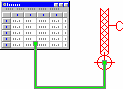
When files are to be used, it is still necessary to draw the problem in the WindTrax interface, as always, by placing wind and concentration sensors, etc. on the map. Files are added to the project by placing input file (spreadsheet) and output file (data logger) icons on the map:

Once placed, the user specifies the details of their file structure e.g. which columns contains the actual input or output values (such as S, C, etc.) (see Using data files in the User's Guide). As file columns are associated with data for objects on the map, connecting cables will appear:

Whatever data is not supplied from data files will, as usual, be taken from its map value. For example, if the surface roughness length or height of your concentration sensor did not change during your measurements, they do not need to be specified in a file, since their values will be obtained from the objects on the project map.

Back to generating the answer

---

WindTrax Output

In most cases WindTrax is used to predict either C or Q. When operating in interactive mode the user can see these predictions by clinking on either the source or the sensor (after the LS model has run). Along with the predicted value of C or Q, a 95% confidence interval is displayed. The LS dispersion model used in WindTrax is a stochastic model, which by definition includes a level of statistical uncertainty. This uncertainty is represented by the confidence interval (CI, calculated using a t-distribution): the LS model estimates the true value of C (or Q) lies in the interval C CI with 95% confidence. The magnitude of CI can be misleadingly low to an experimentalist. Observational uncertainties and the underlying model inaccuracy (e.g. any inaccuracy in the MOST wind relationships) are not included when calculating CI. These factors would introduce additional uncertainties.

The value of CI is to provide a warning for situations where WindTrax predictions are prone to large errors. A large CI can occur because: 1) the LS model has not used enough particles in the simulation, or 2) the wind direction is such that only a small fraction of model source material arrives at a concentration sensor. The uncertainty can generally be reduced by increasing the number of LS model particles (see key LS model variables).

In certain cases WindTrax cannot make a prediction because the meteorological conditions prohibit a solution. The often occurs in a Q-inference problem. If the concentration sensor is outside the source area, then in some cases the wind direction means the concentration sensor cannot "see" material from the source, so no prediction of Q is possible. In this situation WindTrax will output a Q value of -9999 to an output file, or will report "Estimate not valid" on the screen.

Unexpected results

Back to WindTrax introduction

---

The LS dispersion models

The basis of the WindTrax analysis is the dispersion model prediction of the Q-C relationship between tracer sources and concentration sensors. Any type of atmospheric dispersion model could be used to give this relationship. In the hierarchy of dispersion models, the Lagrangian stochastic (LS) approach is the most natural and. In an LS model, the trajectories of thousands of tracer "particles" are mimicked as they travel through the turbulent air. There are two types of LS models. Forward models follow particles downwind from the emission source to a concentration receptor (volume surrounding the concentration sensor). Backward models (BLS) follow particles upwind from the concentration sensor to the emission source. WindTrax has been designed to take advantage of computational efficiency of the BLS model.

Backward LS (BLS) model
Touchdown catalogs
How WindTrax uses the Touchdown Catalog library
The BLS procedure using a line-averaging sensor
Key LS model variables

Back to WindTrax introduction

---

The Backward LS (BLS) model

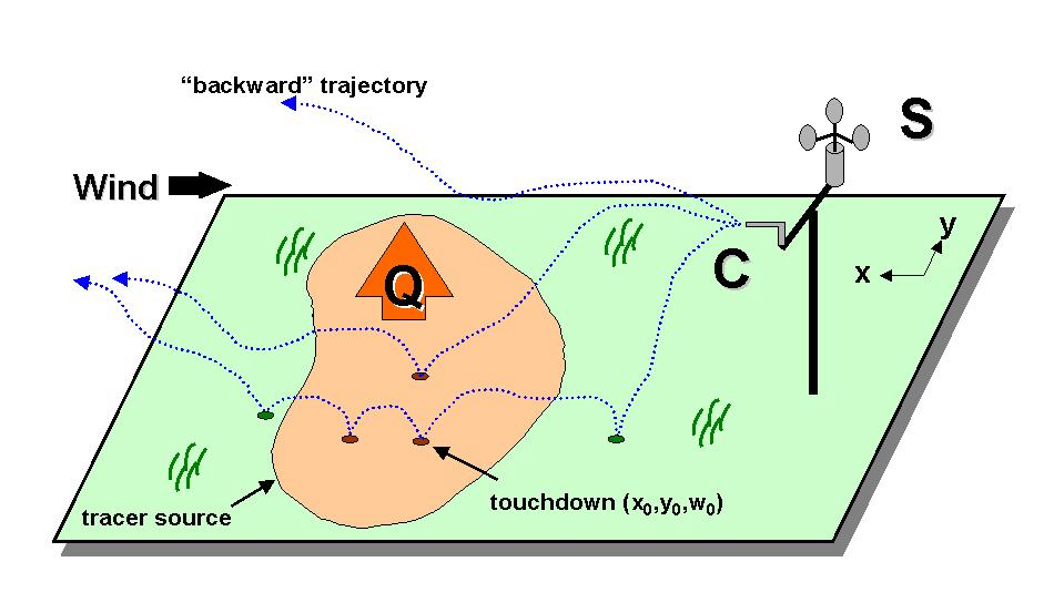
For surface area sources the backward (or "inverse") LS approach is a particularly efficient way of determining the Q-C relationship. In a backward LS model (BLS), the upstream trajectories of tracer particles are calculated from a release point at the site of the concentration sensor. The crucial trajectory information is the touchdown locations (x_o,y_o) and the vertical "touchdown" velocities (w_o) when trajectories "impact" the ground within the source region. The attraction of the BLS method (besides accuracy of the underlying LS model) is the ease with which complex source sizes and shapes can be simulated, and the computational efficiency of the method. Although WindTrax will use a forward LS model to calculate C/Q for point sources, it was specifically built to take advantage of the BLS method.

When WindTrax is calculating C/Q for area sources, the user sees pinpoint dots being placed on the WindTrax map. These are the touchdown locations of the backward trajectories. These touchdowns proceed from the concentration sensor in an upwind direction. As the touchdowns are displayed WindTrax is separating touchdowns which occurred within the source area from those outside the source. The complete field of touchdown locations and touchdown velocities is called a touchdown "catalog".

Touchdown catalogs

Back to dispersion models

---

Touchdown Catalogs

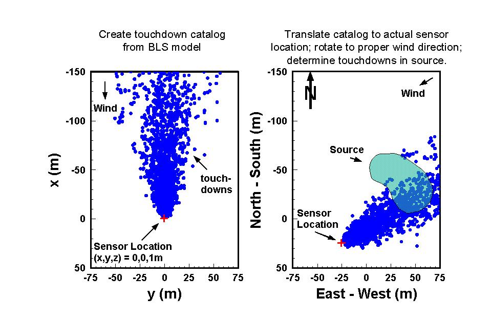
One advantage of the BLS approach is the ability to pre-calculate touchdown catalogs without any knowledge of the eventual source size and location. This is because source information is not needed to create the necessary touchdown field. Only after the touchdown catalog has been created is source information utilized. Adding to the utility of a touchdown catalog are the following:

1. Touchdown locations (x_o, y_o) do not change with changing windspeed. This is because of the way turbulence properties in the ASL scale with windspeed.
2. Touchdown locations can be horizontally translated to any sensor location (in horizontally uniform conditions).
3. Touchdown locations can be rotated to any wind direction (in horizontally uniform conditions).

For a given Z_o and L (and concentration measurement height z_c), a single touchdown catalog will describe any future problem. Once a source is defined, and windspeed and wind direction measured, the pre-calculated touchdown catalog is translated and rotated to the sensor location and proper wind direction, and the touchdowns mapped. Only touchdowns within the source are used to calculate C/Q. A key feature of WindTrax is the ability to use pre-calculated touchdown catalogs.

How WindTrax uses touchdown catalogs

Back to dispersion models

---

How WindTrax Uses the Touchdown Catalog library

Using pre-calculated touchdown catalogs dramatically increases the computational efficiency of WindTrax. An important part of WindTrax is managing and identifying previously calculated touchdown catalogs - the touchdown catalog "library". When confronted with a new problem, WindTrax checks the catalog library to see if a catalog exists which corresponds to the problem at hand (i.e. the same Z_o, L, and the concentration measurement height z_c). If a matching catalog exists, then WindTrax uses it. WindTrax comes with an initial library of over 500 catalogs on CD.

The are several choices the user makes regarding how WindTrax utilizes the catalog library. These are to set the tolerances for Z_c, Z_o, and L when deciding whether WindTrax should use a pre-existing library catalog, or generate a new catalog. These choices allow the user to balance computational efficiency against model accuracy.

The first choice is to select a tolerance for the height of the concentration measurement Z_c (see setting the Z_c tolerance). WindTrax will use the tolerance criterion to decide whether to use a pre-existing catalog from the catalog library. Suppose the user has a problem where Z_c = 2.0 m. If the user selects a tolerance of 10%, then WindTrax will use a touchdown catalog created for Z_c = 1.85 m if it exists (and if it further matches the Z_o and L for the problem). The default setting is 10%.

The next choice is to decide if WindTrax should:

• Use standardized values for Z_o and L. In this option, WindTrax "bins" the specific Z_o and the L values into one of these categories:
  
  

  If Zo in this range	Use this Zo		If L in this range	Use this L
  Zo < 0.0003 m:	0.0001 m		0 m < L < 10 m:	L = 5 m
  0.0003 m < Zo < 0.0014 m:	0.001 m		10 m < L < 40 m:	L = 20 m
  0.0014 m < Zo < 0.003 m :	0.002 m		40 m < L < 300 m:	L = 100 m
  0.003 m < Zo < 0.007 m:	0.005 m		L > 300 m; L < -300 m:	L = 1010 m
  0.007 m < Zo < 0.014 m:	0.01 m		-300 m < L < -40 m:	L = -100 m
  0.014 m < Zo < -0.03 m:	0.02 m		-40 m < L < -10 m:	L = -20 m
  0.03 m < Zo < -0.07 m:	0.05 m		-10 m < L < 0 m:	L = -5 m
  Zo > 0.07 m	0.10 m

  The reason for using the standardized values is to dramatically increase computation speed. Using standardized values greatly reduces the number of catalogs required for a broad range of problems. For a given measurement height, a total of 7x8 catalogs cover all circumstances. This means the user is more likely to have a useable catalog in their catalog library, and therefore spend less time generating new catalogs. The scientific rationale for "binning" Z_o and L is that Z_o and L are difficult to measure with much precision (20% would be a maximum), so that a subdivision of Z_o and L beyond the above range is not warranted.

• Use selected values for Z_o and L. In this option the user selects tolerance criteria for Z_o and L to use when selecting a catalog from the catalog library. These are specified in percentages (see selecting Z_o and L tolerance). If WindTrax finds a pre-existing catalog within the selected tolerances, it uses that catalog. The default values are 10%.
  
• Use exact values for all variables as determined from the available wind field measurements.

Back to dispersion models

---

The BLS Procedure Using a Line-averaging Sensor

A line concentration sensor calculates tracer concentration in a line between two points. An example is an open-path laser system, which measures concentration along the laser path. A line sensor is a good match with WindTrax. Using a horizontal line average reduces the sensitivity of model predictions to errors in the BLS model. The accuracy of the BLS model in predicting horizontal dispersion is not as critical in this case compared with a point concentration measurement.

Using the BLS method with a line-average concentration follows the same procedure as for a point measurement. The difference is how the touchdown catalog is applied -- not to estimate a single point concentration but a line average.

Back to dispersion models

---

Key LS Model Variables

For most users the internal details of the LS dispersion model are not important. We have tried to keep most of the intricacies hidden. However, there are two key variables that the user should be aware of, and may need to change.

The most important detail is the number of "particles" used in the LS model simulations (N). Typically N = 10,000 to 50,000 particles. In any given situation, the larger the value of N, the lower the model uncertainty. When the source region decreases in size, or when the concentration sensor becomes more distant from the source, a larger N is often required (see selecting N). It may also be necessary to increase N if the concentration sensor is located near the edge of the tracer plume emanating from the source. There is larger uncertainties in the LS model predictions near the plume edge (i.e. fewer model particles occur at the edge of the plume). In some cases increasing N does not decrease the model uncertainty. If the concentration sensor is outside the source area, and the wind direction is away from the sensor, no prediction of Q is possible. Increasing N has no effect.

The other important LS variable is particle-tracking distance. When WindTrax calculates a touchdown catalog it tracks particles for a distance X upwind. X must be larger than the furthest point the source is away from the sensor where C is observed or predicted. WindTrax automatically calculates X for a given problem. The selection of X is not just determined by the problem at hand. The greater the value of X the greater the utility of a catalog: a catalog with a large X will be useful for many problems, while one with a small X has limited potential. The user may therefore select a larger value of X than needed for a problem in order to increase the usefulness of that catalog (see selecting tracking distance).

The tracking distance X should generally not exceed 1000 m. This means WindTrax should not be used for problems where the source-sensor scale is greater than 1000 m. The reason lies in the accuracy of the LS model. The LS model in WindTrax is valid for the ASL, which is the lowest 50-100 m of the atmosphere. To track tracers beyond 1000 m in principle requires model accuracy above a height of 50 m: material transported beyond 1000 m may have been transported above 50 m. The argument is that if WindTrax does not accurately simulate transport above 50 m, it cannot make accurate predictions beyond 1000 m. We believe the 1000-m maximum scale is conservative.

Back to dispersion models

---

Sources of error and uncertainty

We can divide the uncertainties associated with the results provided by WindTrax into two categories:

• Those associated with the accuracy of the LS model;
• Those associated with uncertainties in field measurements.

Back to introduction

---

Larger Nighttime Uncertainties

For homogeneous flat terrain, in typical daytime conditions, there is little doubt as to the accuracy of LS dispersion models. Potential problems are poor representation of nighttime conditions, and flow obstructions. The stable nocturnal boundary layer is a problem because the atmosphere may not follow the same simple set of "rules" as during the day. At night the atmosphere is often in a complex state of transition. The ability of dispersion models to accurately describe nighttime conditions is limited. Therefore as a general rule, WindTrax predictions will have greater uncertainties at night.

Non-ideal experiment site
Back to sources of error

---

Non-ideal Experiment Site

At some locations the accuracy of LS models is compromised by "flow obstructions". If a source is situated close downwind of a barn for instance, then the atmosphere will be "disturbed" by the barn, with different wind characteristics than found at a flat site. This leads to errors in WindTrax. While it is theoretically possible to handle this complexity (although not in WindTrax at the present), it is a very difficult problem.

As a rule of thumb, tracer sources and sensors (as well as meteorological sensors) should be at least 10 obstruction heights away any obstruction. This rule specifically applies to upwind obstructions (as downwind obstructions have limited effect). In some settings this means certain wind directions allow for accurate WindTrax predictions, while other wind directions give unusable data.

Our experience to date suggests that irregularity caused by minor undulations of the terrain, or widely-scattered low obstacles to the flow (such as weeds or shrubs), do not invalidate WindTrax.

Back to sources of error

---

Uncertainty in field observations

Inaccurate wind speed (S) measurement
Inaccurage Z_o measurement
Inaccurate Obukhov length measurement
Inappropriate averaging time
Poor placement of concentration sensor
Additional Tracer Sources - Background Concentration

Back to sources of error

---

Inaccurate S Measurement

WindTrax requires an accurate measurement of windspeed S, and this is not without difficulty. In general, the relative error in S translates into a similar relative error in either Q or C: a 10% error in S leads to roughly a 10% error in the inferred Q or C.

Cup anemometers are the standard for S measurement, and they are susceptible to stalling (stopping in low winds) and overspeeding (overestimating the windspeed in turbulent conditions). In most cases stalling is a more serious problem. This most often happens at night and at low measurement heights. An advantage of WindTrax is that S can be measured at any height. A high location can be chosen where there is less chance of stalling.

Note: WindTrax will not run with S = 0.

Back to measurement uncertainties

---

Inaccurate Z_o Estimate

Surface roughness Z_o is difficult to measure. It is subject to inaccuracies in S observations, non-ideal terrain, and inaccuracies in the theoretical logarithmic wind profile that defines Z_o. It is often sensitive to wind direction (i.e. the upwind environment) and S. We often see substantial variation in Z_o from one 30 minute period to the next.

There is no fixed rule relating uncertainty in Z_o to uncertainty in the WindTrax predictions. The relationship depends on the size and shape of the tracer source, the location of the concentration sensor, and atmospheric stability. While there are some situations where there would be sensitivity, our experience has generally been that there is not great sensitivity to Z_o.

Given the measurement difficulties in measuring Z_o, we believe the value of Z_o can be taken from literature values where measurements have been taken over similar terrain. The error in using literature values should not be much greater than the typical uncertainties of field estimates of Z_o.

Back to measurement uncertainties

---

Inaccurate Obukhov length measurement

The value of L changes from half-hour to half-hour, and it is the most difficult meteorological input to measure. How sensitive are WindTrax predictions to L errors? There are no fixed rules about this. The sensitivity depends on the size and shape of the tracer source, the location of the concentration sensor, and atmospheric stability. There are some situations where a mis-classification of stable to unstable will result in more than a 50% error in the C or Q prediction. Usually the sensitivity to stability increases as the source size decreases.

As a general rule we would say that it is important to accurately separate stable, near- neutral, and unstable situations. Less important is the degree of sub-classification from this tri-class. It is important to recognize that even with rigorous measurement techniques, it is doubtful L can be measured to better than about 20% (assuming u_* measured to order 5%, heat flux to order 5%). Furthermore the micrometeorological formulae that exploit L are best fits to scattergrams, with substantial uncertainties.

The message here is that you should definitely worry about whether a situation is unstable, stable, or near-neutral. More precision than this is certainly desirable. However, you should worry progressively less about separating L with increasing precision.

See also:

  Measuring L Directly
  Estimating L From a Richardson Number
  Estimating L and z0 from S and T Profiles
  Estimating L from the Standard Deviation of Wind Direction

Back to measurement uncertainties

---

Appropriate Averaging Time

How long should the averaging interval (measurement interval) for C and S be? The LS model in WindTrax is used to predict time-average properties of the atmosphere, and errors can result when inappropriate time intervals are used. We can only expect the predictions of an LS model to be valid over a comparable time-frame as used in the internal statistical description of the atmosphere in WindTrax. The model relies on the typical micrometeorological description of the atmosphere -- based on (roughly) 30-minute statistics of the atmosphere. The logical conclusion is that WindTrax should be applied to order 30-minute average data (certainly not 10-second data, nor daily data).

The most defensible approach is to use 30 minute or shorter averaging periods. How short an averaging time can be used? Flesch et al. (1995) found averaging periods down to 1 minute gave good results in one study. However, we would not advise less than a 5 minute averaging time.

Back to measurement uncertainties

---

Poor Placement of Concentration Sensor

Inaccuracy can result from poor placement of the concentration sensor. The LS model is more accurate predicting the C-Q relationship at locations near the center of the plume rather than at the edge of the plume. The reason is two-fold. First, the model is more accurate because larger numbers of model particles pass near the plume center, and results in a more precise sampling of concentration. The second reason is that plume-edge features are often the result of rare and extreme events. Like all environmental models, WindTrax has difficulty simulating extreme events.

This ramification of this is that the user should take care not to place the concentration sensor in a spot which guarantees a plume-edge position. This commonly occurs when the sensor is placed too high in relation to the source plume. For example, if the source is a square 5 meters on a side, and the concentration tower is placed at the center of the square, then a measurement height of z = 1.5 meters is outside the densest part of the source plume. If possible the sensor should be moved down.

There are no rigid rules for placing the concentration sensor. Experience is usually the best teacher. However, as a start we suggest that if the sensor will be placed within the source boundary, that a sensor height of 20% of distance from the sensor location to the upwind edge of the source is appropriate.

Back to measurement uncertainties

---

Additional Tracer Sources - Background Concentration

Sometimes the identified emission sources are not the only source of tracer. The existence of distant sources, which result in a uniform background concentration (C_bg) is not a large problem for WindTrax if C_bg can be measured. In WindTrax a background concentration sensor can be placed on the map and C_bg entered.

A more difficult problem arises with nearby undefined tracer sources. These result in a C_bg that varies with location. This means a problem with intermingling of separate evolving tracer plumes, and the apportionment a C observations to a specific source is not generally possible.

Back to measurement uncertainties

---