WindTrax User's Guide
This guide is intended to assist you to accomplish the basic tasks of designing, creating, editing, and running WindTrax simulations. It is divided into the following sections:
- Tools
- The map grid
- Sensors
- Sources
- Using data files
- Project status
- Running simulations
- Numerical models
- Miscellaneous objects
- Changes from WindTrax version 1 to 2
 WindTrax tools
WindTrax is equipped with a number of tools for drawing and editing the project map. These can be accessed either through the tool buttons above the map or by selecting from among the items in the main menu. The tools are grouped according to function (View, Edit, Actions, Platforms, Sensors, Shapes, Data, and Miscellaneous) on separate tabbed tool bars located above the map.
Only one tool is active at any time. The name of the tool being used is displayed on the status panel at the bottom of the main window; in general, its button will remain down while it is in use. The only tool available while a simulation is running is the Query Pointer.
With some exceptions, each time a tool is used once, the active tool returns to Pointer. To override this behaviour, hold down the <Shift> key while clicking any tool; it will remain active until another is selected.
Tool classificationsBack to User's Guide
Tool classifications
WindTrax tools might be classified into four groups:
Back to User's Guide General tools
The following tools of general use are available:
- Pointer
- Query Pointer
- Rotate
- Rescale
- Map Grid
- Tape Measure
- Paint Can
- View Menu Item
- Select Menu Item
- Zoom
- Map overview form
- Magnifying glass
Pointer map tool

The Pointer is the default map tool; it allows you to select, move, resize, and redefine parameters of objects on the map. To select an object, click it once; this will cause a highlight rectangle to appear around it. To select a group of objects, either hold down the Shift button while clicking on individuals, or press the mouse button down over the background, and drag the mouse to form a selection rectangle. Release the mouse to select all objects within the rectangle. Once objects are selected, they can be moved, deleted, or modified through their property editor. To access the property editor form, double click any object (including the background) on the map with the Pointer tool or on its name in the Object List form.
It should be noted that any objects moved off the project map and then unselected will be deleted automatically. This is necessary in order to prevent projects from becoming unusable due to hidden and inaccessible objects.
Back to general toolsMoving objects with mouse and keyboard
Objects on the map can be moved in either of two ways:
- grab the object by moving the mouse pointer over the object to be moved, pressing down the mouse button, and moving the mouse while holding the button down.
- first, select the object (either with the mouse pointer or by pressing <Tab> on the keyboard); then move the selected object one pixel at a time by holding down <Ctrl> and using the arrow keys.
Query Pointer map tool

The Query Pointer provides quick access to the data and state of any object on the map; it is the only tool available during and after a simulation run. In the normal edit mode, the Query Pointer will display information about the object which has been clicked with the mouse; the information will remain visible only as long as the mouse button is pressed.
During a simulation, the Query Pointer shows the present state of any object at the present moment. When the simulation is completed, clicking any object will show the results for the selected object. Information will remain visible until clicked by the pointer; in the case of output data files, the output file will be displayed and remain until the edit window is closed.
Back to general toolsRotate map tool

The Rotate tool allows you to select and rotate collections of objects about an adjustable pivot point. To do this, click the Rotate button on the Edit tool bar. The rotation angle relative to the grid can be specified in the edit box visible at the top of the map when the Rotate tool is active.
Back to general toolsRescale map tool

The Rescale tool allows you to select and resize collections of objects about an adjustable central location. Rescaling allows the user to quickly adjust the relative size of all objects on the map, while retaining their geometric relationships. To do this, click the Rescale button on the Edit tool bar. The scaling parameter can be specified in the edit box visible at the top of the map when the Rescale tool is active.
Back to general toolsMap Grid tool

The Map Grid tool is used to adjust two features of the grid defining locations on the project map:
Back to general toolsSetting the location of the grid origin
To change the location of the map origin, either select Map|Origin from the main menu; click on Map Grid in the Object List form; or click once on the Map Grid tool button found on the Edit tool bar to highlight the origin. To move it, use the arrow keys or drag the origin with the mouse to its new location. By default, the map tool will automatically be reset to the Pointer when the mouse is released; to override this, hold the <Control> button down while moving the origin.
The default location of the origin can be changed by selecting Tools|Environment from the main menu and setting a new location (in pixels) on the main map.
Back to map grid toolSetting the grid scale
To set the map scale, either double click the Map Grid button on the Edit tool bar above the map; or select Map|Grid from the main menu; or double click on the name Map Grid in the Object List form. The scale selected should be one which is convenient to use yet allows the entire simulation to be represented within the base map area. (The default value, set at 2m, can be changed by selecting Tools|Environment from the main menu, and choosing a new default scale distance.)
Back to map grid toolTape Measure map tool

The Tape Measure has two main functions: first, it performs distance measurements between any two points on the project map, in the units of the present scale; and second, it allows you to define the map scale based on a known distance measurement. This tool can be activated either by clicking on the Tape Measure button on the Edit tool bar, or by selecting Draw|Tools|Tape Measure from the main menu. To use it, press the mouse button down at the starting location, drag the mouse to the end point, and then release the button.
The edit box appearing at the top of the map can be used to redefine the current distance measurement, and redefine the scale accordingly. The same approach can be used when drawing a line sensor or geometric shapes (rectangles and ellipses).
Back to general toolsPaint Can map tool

The Paint Can is used to change the colour of shapes on the map. To use it, press the Paint Can button on the Edit tool bar located above the map, or select Draw|Tools|Paint Can from the main menu. The active colour is selected by clicking on the Colour Palette, which appears below the main tool panel. Any shape that is clicked with the mouse cursor (which should now look like a can pouring paint) will change to the currently active colour.
Back to general toolsSpecial paint can modes
Two special modes exist for the Paint Can map tool:
- If the mouse button is clicked while <Ctrl> is held down, all shapes of the colour under the cursor will change to the active colour.
- If <Shift> is held down, all shapes beneath the cursor, of any colour, will change to the active colour.
Changing the background colour
In order to change the colour of the background map, double click on the background using the Pointer tool to show the surface data editor, and click on colour. The default background surface colour can be set by choosing Tools|Environment from the main menu.
There is only one constraint on the choice of colour for the base map surface: it cannot match any of the source colours. If one of these is selected, an error message will appear. If your intention is to simulate an infinite source, this can be only approximated by drawing a sufficiently large shape of the desired colour.
Back to paint can toolView menu item
The View menu item allows you to hide or reveal various types of objects on the map; this can be useful in editing or when working with an object which lies under a number of other objects. To determine which objects are visible, select View from the main menu and choose an object type e.g. area source.
Back to general toolsSelect menu item
The Select menu item permits you to select or unselect all objects of a given class. It is particularly useful when working with large objects occupying most of the map space; when access to the map surface to unselect objects is difficult; choosing Select|Unselect All from the main menu will do that.
Back to general toolsZoom In/Zoom Out


The apparent distance from the WindTrax map can be changed using the Zoom In and Zoom Out tools. To select the tools, click the Zoom In or Zoom Out buttons found on the View tool bar, or select View|Zoom In or View |Zoom Out from the main menu. Move the cursor to the location you want to be centered when the magnification change occurs, and click the mouse button. If the <Shift> key is held down while the mouse button is pressed, the zoom tool will remain active; otherwise, the Pointer tool will be retrieved automatically.
The map can be magnified by up to eight times. When this is done, the pixelized nature of the shapes will become apparent.
Back to general toolsMap Overview form
The Map Overview form provides a miniature view of the entire map, in which the portion presently visible is highlighted by a rectangle. This can be useful for navigating around the map when Zoom is larger than one. The view port can be moved to another location by holding down the <Control> key and dragging the highlight rectangle with the mouse. If <Control> is not held down, the Map Overview form will itself be moved.
The form can be hidden either by selecting View|Map Overview from the main menu, or by right-clicking on the form and selecting Close from the popup menu. By default, the Map Overview form is not visible when WindTrax is first loaded; this can be set using the Tools|Environment main menu item.
Back to general toolsMagnfying glass
When working with sensors and other objects, it is sometimes convenient to have a close-up view of the cursor's location. This is provided by the Magnifying Glass, which can be shown or hidden by either clicking on the Show Magnifying Glass button on the View tool bar at the top of the map, or by selecting View|Magnifying Glass from the main menu. At any time it can be hidden in the same way. Its location can be moved to wherever is convenient, by grabbing it with the mouse.
Back to general tools Edit tools
The following tools, located on the Actions tool bar at the top of the map, are used in editing the features on a map:
- Copy
- Paste
- Cut
- Delete
- Merge/Unmerge
- Bring to Front/Send to Back
- Lock/Unlock Positions
Delete

Delete removes an item from the project. To remove one or more selected objects from the map permanently, you can do one of several things:
- click the Delete button on the Actions tool bar;
- select Edit|Delete from the main menu;
- type <Ctrl Delete>;
- right-click on one of the objects and select Delete from the popup menu.
Any map objects that are moved off the project map and then unselected will be deleted automatically.
Back to editing toolsMerge/Unmerge


Merge allows you to group two or more shapes so that they will behave as a single object. Select the shapes using the Pointer tool, and then click the Merge button on the Actions tool bar; select Edit|Merge from the main menu; or type <Ctrl M>.
Unmerge will ungroup previously grouped shapes. Select the merged shape using the pointer to, and then click the Unmerge button, select Edit|Unmerge from the main menu, or type <Ctrl U>.
Back to editing toolsBring to front/Send to back


Bring to Front moves one or more objects of a given type so that they appear in front of the others of its type. To do this, select the objects using the pointer tool and then click the Bring To Front button on the Actions tool bar; select Edit|Bring to Front from the main menu; or type <Ctrl F>.
Send To Back moves one or more objects of a given type behind all others of its type; select the objects using the pointer tool and then click the Send to Back button on the Actions tool bar; select Edit|Send to Back from the main menu; or type <Ctrl B>.
Back to editing toolsLock/Unlock positions


To prevent objects from moving when editing their properties, click the Lock button on the Actions tool bar, select Edit|Lock Positions or type <Ctrl L> to lock their position on the map. To unlock positions and again allow objects to be moved, repeat the procedure. Note that locking positions is a global feature; all objects will be locked, not just those being edited.
Back to editing toolsMap objects
WindTrax project consist of a number of different objects, most of which you will have add to the map. These objects include:
- The map grid
- Sources
- Sensor Platforms
- Sensors
- Data Objects
- Imported images (bitmaps and jpegs)
- Miscellaneous objects
Common map object features
Although they have different uses and properties, all objects on the map share many features in common, such as names, most of which can be changed, and an Enabled property which allows them to remain on the map but not take part in the simulation.
Working with map objects is much the same for all of the different types. Each can be:
- created, by selecting a particular tool and then creating a new object by clicking on the map;
- selected, by clicking the object with the Pointer tool; by typing <Tab> or <Shift Tab> on the keyboard; or by clicking on the object's name in the Object List form
- moved, rotated, or rescaled using either the Pointer tool or the keyboard;
- deleted, by selecting the object and clicking the Delete button; selecting Edit|Delete from the main menu; right-clicking on the object and selecting Delete from the popup menu; or typing <Ctrl Delete>.
- enabled or disabled, which allows you to temporarily remove an object from the map without permanently changing its data.
In addition, any object (including the background surface and map grid) can have its data or properties:
- edited, by double-clicking with the Pointer tool, or double-clicking on the object's name in the Object List form, to reveal a property editor form suited to the object;
- displayed at any time using the Query Pointer.
Object List form
The Object List form provides a list of the names of all editable/viewable objects in the current project. By clicking or double-clicking with the mouse over any name in the list, the object's data can be edited and/or viewed.
Clicking the mouse will cause the object to be highlighted on the map; while the simulation is running, its present state will be displayed.
while in edit mode, double-clicking the mouse over an object's name will cause its property editor to be displayed.
At any time, the Object List form can be shown or hidden by clicking the Object List button on the View tool bar; selecting View|Object List from the main menu or by typing <Ctrl-Alt-O>.
Back to map objectsTouchdown catalog utilities
In order to speed up backward LS model calculations, it is possible to store the locations and vertical velocities of particles as they reach the surface in their flight. The catalogs will differ based on their particle number, time scale ratio, release height, surface roughness length, stability, and horizontal tracking distance (for more details about these terms, consult the help on the LS models). These files, referred to as Touchdown Catalogs, will be generated automatically by the LS model whenever a suitable match amongst the existing catalogs cannot be found. A set of over six hundred of these files is included with the WindTrax software, in the directory Catalogs on the CD.
Two utilities are included to assist you in managing and creating these files:
- the Catalog Manager
- the Catalog Generator
Catalog Manager
Touchdown catalog files are stored in a binary format, and are therefore not legible directly. In order to allow you to examine the parameters associated with each file, and to manage the large number of files potentially generated, a Catalog Manger tool is included with WindTrax. It is accessed by selecting Tools|Catalog Manager from the main menu.
The manager displays the properties (such as size, number of particles, release height, etc.) of all catalogs on the CD and in the default Catalogs directory, which is used to store newly created catalogs. From the manager, it is possible to select and delete these files (other than those on the CD).
At the end of each session, you will be asked whether or not you wish to save the catalogs generated during that session. By selecting Tools|Environment from the main menu, this can be changed.
Back to TD catalog utilitiesCatalog Generator
The Catalog Generator is a utility intended to permit you to create touchdown catalogs without running a particular simulation. It can be accessed by selecting Tools|Catalog Generator from the main menu. After selecting the parameters for a set of catalogs, a file for each of the seven standard stability categories will be generated in the background, while you are free to do other tasks.
Back to TD catalog utilitiesMap grid and orientation
Each project in WindTrax has an associated grid, scale, origin, and geographic orientation, allowing you to specify the geometry of the simulation.
Grid, scale, and originMap orientation
Effects of pixelization on the grid
Back to map objects
Grid, scale, and origin
The map grid is the set of dotted gray lines that appear when WindTrax is loaded. It can be shown or hidden using either the button on the View tool bar at the top of the main window or by selecting View|Grid from the main menu. The spacing (in pixels) between its lines, which represents the map scale, can be changed by accessing the map grid's property editor; see Map Grid tool. The default value, 20 pixels, can be set by selecting Tools|Environment to display the default settings page.
The map scale is shown on the status bar at the bottom of the main WindTrax window, and represents the perpendicular distance between the grid lines. The scale is set using either the Map Grid tool or the Tape Measure tool. To change the location of the origin, click once on the Map Grid tool button or select Map Origin from the main menu to select the origin; then drag it to its new location. To return to normal edit mode, select any other tool.
As the mouse moves over the project map, its location is displayed in units of distance in the status panel at the bottom of the main window.
Back to map gridEffect of pixelization on the map grid
Because the map is divided into a finite number of pixels, there is a subtlety involving the precise location and meaning of the grid lines and their relationship to map objects. In particular, the map grid lines are assumed to be located at the center of the pixels in which they are drawn, and not their edges. Similarly, the map origin and all point sensors are assumed to be located at the center of the pixel at the focus of their cross-hairs. Shapes, however, are drawn so that the edges of their extent correspond with the edges of the pixels in which they are drawn. There will therefore be an offset of one half pixel width between the grid and any shapes drawn on the map. If the shapes are large enough to be a good representation of the source, the effect of this offset should be small. For further information, consult the help on pixelization of shapes.
Back to map gridMap orientation

By default, geographic North is assumed to be at the top of the map. This can be changed through the North Indicator, which can be shown or hidden either by clicking the View Compass button on the View tool bar or by selecting View|Compass from the main menu. To change the orientation of the map grid, double click on the compass or select Map|Orientation from the main menu.
Back to map grid Sensors
In the real world, we require specialized sensors to measure meteorological variables (e.g. temperature, pressure, wind speed, tracer gas concentration). In general, this is true in WindTrax as well; for any quantity the user wishes to include in a simulation, a suitable sensor must be present on the map. The following topics will discuss sensors and their use in detail:
Sensor output modeSensor platforms
Sensor types
Working with sensors
Back to map objects
Sensor output mode
There is a key difference between actual sensors and those used in WindTrax: sensors in WindTrax can either provide measured values or request that they be calculated. These two possibilities will be referred to as output modes. Sensors that you provide with specific key data will be said to be in given mode; these will be used as boundary conditions for the underlying models. Sensors used to request and receive a model-determined result will be referred to as being in unknown mode.
Some sensors, such as the IHF sensor, can be in unknown mode only i.e. cannot specify a known value. The mode of a sensor may depend on the type of platform to which it is attached: profile, contour, cross-section, and transect plots cannot be used to provide boundary conditions to the model, so any sensor attached to them will be changed to unknown mode automatically. You can specify which output mode a sensor has on its editor form. For further information, see Setting sensor output mode.
Back to sensorsSensor platforms
Another similarity to real sensors is that any sensor we might require in WindTrax must be placed on some type of platform, such as an instrument tower. The output mode and number of measurements made by a single sensor will depend on the type of platform to which it is attached.
Types of sensor platformPlacing a sensor platform
Back to sensors
Types of sensor platform
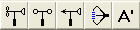
The following three categories of platforms are available at present:
- Point platforms (tower and truck)
- Line platforms (laser, mulit-path, and multi-point)
- Plotting platforms (vertical profile, horizontal and vertical contour, and transect)
Point sensor platforms


The two point platforms (tower and truck) are the simplest of those available; sensors attached will provide a single measurement, at a specific location, and can be in either given or unknown modes. Towers are the default platform; if a sensor is placed on the map without a platform beneath the cursor, a tower will be created for it automatically. The truck platform permits you to specify the coordinates of its location from a data file so that the sensor can move around during the simulation.
Back to sensor platform typesPlot sensor platforms


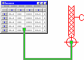
![]()
The four plotting platforms (vertical profile, horizontal contour, vertical contour or cross-section, and transect) allow you to measure values along a straight line or on a two-dimensional grid of locations (horizontal or vertical). Sensor attached to these platforms can be in unknown mode only and will be converted automatically; this means that sensors attached to plots cannot accept input data and cannot be used to provide model boundary conditions.
Working with profile and transect plotsWorking with the contour plots
Back to sensor platform types
Working with profile and transect plots
There is an important practical consideration when using profile or transect plots to observe concentration along a straight line: for each height, a new touchdown catalog will be required for the backward LS model. For those heights at which catalogs have already been calculated, this is not an issue; yet a significant number of new catalogs could be required, particularly if the sensor height tolerance has been set low in the backward LS model. The bottom line is that it could take a lot of time and disk space to do this. Use such plots judiciously to reduce this overhead.
The transect plot, new to Version 2.0, is useful for observing concentration along a line of interest; for example, along the downwind axis of a point source plume. It requires much less computational overhead than the contour plots. To add a transect plot to the map, click on the Transect Plot button on the Platforms tool bar. Click on the map where the start should be located and then drag the mouse until the cursor is over the end location.
Add sensors to the platform by clicking on a sensor tool button, then clicking on either end of the transect plot (i.e. not along the line joining the two). Alternatively, double-click on the plot and click the Add Sensor button on the Sensors page. Its position can be adjusted by dragging the ends with the mouse. If grabbed by the outer square, the entire plot will move; by the inner square, only the local end will move.
Back to plotting platformsWorking with the contour plots
To select and modify the horizontal contour plot, click on the bulls-eye pattern in its lower-right corner. Once selected, the entire plot becomes responsive to the mouse. When adding sensors to the contour plot, they must be placed over the same location.
To select the vertical contour plot, click the mouse over either of its two ends. This will reveal double highlight rectangles over each end. If the plot is dragged from the inner rectangle, only the end grabbed will move; if from the outer rectangle, both ends will move.
The horizontal and vertical contour plot grids are at present limited to 100 points by 100 points; if finer resolution is required, please contact me and I will adjust that.
Back to platformsPlacing a sensor platform
In relation to their placement on the map, sensorplatforms are of two types: point and non-point. To place a point platform (tower, truck, sonde) or profile plot, select the appropriate tool from either the Platforms tool bar or the main menu (Draw|Platform|type); move the cursor to the desired location, and click the mouse button.
To place a non-point platform (contour plot and cross-section plot), select the tool, move the cursor to the desired starting location, and press down the mouse button. While holding the button down, drag the cursor to the desired end location and then elease the button.
The location of all platforms can be adjusted by either dragging the platform with the pointer tool, or by double-clicking on the platform with the cursor to display its property editor and setting the location in grid coordinates directly.
If a sensor is placed on the map in a location where no platform is present, a tower platform will be created automatically.
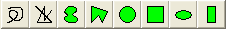
Back to platformsSensor types
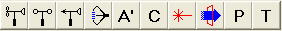
The following sensors are presently available for use:
- Standard anemometer
- Cup anemometer (speed only)
- Sonic anemometer (3-D wind and statistics)
- Wind vane (direction only)
- Wind statistics sensor
- Point concentration sensor
- Line-average concentration sensor
- Integrated horizontal flux sensor
- Pressure sensor
- Temperature sensor
The following sensors were used in earlier versions of WindTrax but are now obsolete:
- Stability sensor (data moved to Surface Layer Model)
- Background concentration sensor (data moved to Atmosphere)
Anemometers
A Standard Anemometer measures both mean wind speed and direction; typically, the values associated with it have been averaged over a fifteen minute to half-hour period. A Cup Anemometer provides (or requests, in unknown output mode) only wind direction, while a Wind Vane measures only wind direction.
In given mode, the Sonic Anemometer sensor accepts data from a real sonic anemometer as accumulated mean values and correlations i.e. <u � u>, <u � v>, <u � w>, <v � v>, <v � w>, <w � w>, <u � T>, <v � T>, <w � T>, and <T � T>. The sonic anemometer accepts data in either raw format (i.e. accumulated average cross-multiplications; e.g. <u � T> = <u'T'> + <u><T>) or variances (raw format minus the cross-multipled means; e.g <u'T'>). Select either Raw averages or Variances/covariances from the Input statistics radio button group on the sensor's property editor form.
For most anemometers, wind speed can be specified in a variety of units; the exception is for sonic anemometers, which accept only m/s for speed and C for temperature units. In WindTrax, a given mean wind speed cannot be specified as zero (though a component of the wind speed can be zero in the sonic anemometer.) In interactive mode, the simulation will not run if this condition exists; when a zero wind speed is encountered in a file, the line will be skipped and flagged as a error. Additionally, the height of an anemometer must be greater than zero.
Wind direction angle is measured either in degrees or radians, east of north, and reports the direction from which the wind is blowing; for example, wind blowing from the north has a direction angle of 0 degrees, while an easterly wind, blowing from the east, has a direction angle of 90 degrees.
Back to sensor typesSonic anemometers
Please contact Thunder Beach Scientific for details on adapting your sonic anemometer to the WindTrax sonic, as the coordinates can be confusing. Many sonic anemometers have different coordinate systems and they may not follow the standard used in the WindTrax sonic: the sensor reports the u wind component as positive when the wind blows towards the East and v is positive when the wind blows towards the North, when the sensor is in its standard position. The software provided by Cerex adjusts the sonic coordinates internally for compatibility, so no changes are required to the standard sensor.
In given mode, the sonic anemometer accepts data in either raw format (i.e. accumulated average cross-multiplications; e.g. <u � T> = <u'T'> + <u><T>) or variances (raw format minus the cross-multipled means; e.g <u'T'>). Select either Raw averages or Variances/covariances from the Input statistics radio button group on the sensor's property editor form. Sonic anemometers accept only m/s for speed and C for temperature units.
Back to sensor typesWind statistics sensor

A wind statistics sensor measures one or more of the ratios σu/u*, σv/u*, and σw/u* in the along-wind coordinate system (i.e. u is in the direction of the mean wind, v is perpendicular to the mean wind, and w is positive upward.) It allows you to override the default values in the particle models and provide measured ratios when they are available This has generally been found to improve the performance of the models.
The ratios are subject to two constraints: they must be positive values and they must satisfy the Schwartz inequalities. In unknown output mode, the wind statistics sensor monitors the ratios being calculated by the surface layer model.
In Version 2, you can add any number of statistics sensors on the map in both given and unknown modes but all but the first given sensor added for each of the three ratios will be ignored unless you over-ride the default behaviour and select them directly. WindTrax can also now calculate the required ratios from sonic anemometer data, so the Wind Statistics sensors are less crucial but still useful if you would prefer to do your own sonic anemometer data analysis. In general, if a sonic anemometer is present, the wind statistics sensor will be ignored. See the Surface Layer Model for further information on the hierarchy of wind sensors. You can opt to enter any subset of the three ratios, by checking only those available on the edit form. Any ratios not provided by any sensors will be estimated from the standard model.
Back to sensor typesStability sensor (obsolete)

You can specify atmospheric stability directly in one of four modes:
- by Pasquill-Gifford Class (symbols A, B, C, D, E, F, or G);
- by General stability class (symbols VU, MU, SU, N, SS, MS, VS, representing Very Unstable, Moderately Unstable, Slightly Unstable, Neutral, Slightly Stable, Moderately Stable, Very Stable);
- by Present Conditions (symbols 0 = bright sunshine, 1 = moderate sunshine, 2 = slight sunshine, 3 = overcast (night or day), 4 = mostly (>= 4/8) cloudy night; 5 = partly cloudy night) (Pasquill, 1961);
- by Monin-Obukhov length L
When stability is specified from a file using any of the first three categories, the symbols in the file must match those listed above.
A stability sensor was used in older versions of WindTrax to specify the state of the atmosphere for use by the default wind model. In Version 2, to access atmospheric stability directly, double-click on the Surface Layer Model icon on the map and select the Parameters tab.
If a sonic anemometer is present, the default action is to calculate stability from the anemometer data; similarly, if a profile of temperature and/or wind speed sensors is present, the default action is to use their data to calculate stability. For further information on stability and how to specify it, see the help on atmospheric stability and the Surface Layer Model
Back to sensor typesPoint concentration sensor

The point concentration sensor, in conjunction with the backwards and forwards LS models, is used to either provide measurements of concentration (when in given mode), from which an unknown source strength can be determined, or to report (in unknown mode) the expected concentration at a location, given a measured (or calculated) set of source emission rates.
Concentration may be specified in a wide variety of units, including parts per million volume (ppm). When ppm or ppb units are used, pressure and temperature measurements must also be provided by the user. In earlier versions of WindTrax, pressure and temperature sensors were added to the map automatically when either of these units was selected. In Version 2.0, you can choose to specify their value either from the default values accessible through the Atmosphere object or by adding temperature and pressure sensors to the map. When a sonic anemometer is present, temperature will by default be specified by its temperature data. If no pressure sensors are available, you can either specify its station value or get WindTrax to estimate it from the surface elevation.
Back to sensor typesLine-average (laser) concentration sensor

The line-average concentration sensor is available for simulating laser-based or open-path UV sensor measurements. Because the line average sensor determines the concentration along a path, its units are in terms of Concentration � Length. This sensor approximates a true line-averaging device by measuring at a series of evenly-spaced points along its length; although the default value is 30 points, the user is free to change this. You can specify up to 52 species of measured tracer simultaneously. The default is an arbitrary tracer whose molecular weight is equal to air. If you are specifying concentration in ppm or ppb, you should select the measured gas species rather than using the default Tracer species.
Back to sensor typesBackground concentration sensor (obsolete)

A background concentration sensor was added to the map automatically in earlier versions of WindTrax. Its function was to report (in given mode) or estimate (if its mode was unknown) the concentration of the tracer gases not originating from any of the sources explicitly added by the user. For Version 2.0, you can access the background concentration by double-clicking on the Atmosphere icon.
WindTrax does not make any checks of the size of the background concentration, other than to require that it is positive if entered by the user. If its value is larger than that which could have been caused by sources on the map, calculated concentrations can be negative.
Back to sensor typesPressure sensor

A pressure sensor was added to the map automatically as required in earlier versions of WindTrax whenever a concentration sensor's units are specified in PPM or PPB. In newer versions, you must add a sensor yourself, or use the station pressure accessible by double-clicking the Atmosphere icon. Pressure can either be specified directly, in a number of units, or estimated from the elevation above sea level of the map. If this option is selected, the pressure is estimated using the hypsometric equation, assuming a constant-temperature atmosphere at 0C.
Back to sensor typesTemperature sensor

A temperature sensor was added to the map automatically whenever required in earlier versions of WindTrax. In newer versions, you have to add a sensor yourself or use the global screen temperature accessible by double-clicking on the Atmosphere icon. Temperature can be specified in either Celcius, Kelvin, or Fahrenheit units; if it outside the normal meteorological boundaries, a warning will be generated. Back to sensor types
Working with Sensors
Sensors in WindTrax have the same behaviours as the other objects on the map: they can be added, deleted, moved, rotated, rescaled, and be edited. The following topics are available:
- Adding a sensor to the map
- Placing a line concentration sensor
- Setting sensor output mode
- Specifying sensor data
- Deleting a sensor
Adding a sensor to the map
There are two approaches to creating a new sensor, of any type:
- click on the Sensors tool button on the main tool panel, or select Draw|Sensor from the main menu and select a sensor type. Move the mouse cursor (which will now appear as a circle with a cross through it) until the cross is over the desired location on the map, and click the button. If no platform is present beneath the cursor, a tower will be created automatically; otherwise, the sensor will be placed on the existing platform. The plot platforms can accept only a single sensor of any given type; they will automatically configure their sensors to measure at each of their grid locations.
- if the platform to which you want to add the sensor already exists, double click on its icon, and then click the Add button on its property editor. Select a sensor type from the list and click OK. If the platform you wish to use is not present on the map, you must first create it, and then follow the procedure as above.
Placing a line concentration sensor
To position a new line sensor on the map, first select the line concentration sensor tool. Move the mouse to one of its end locations (either laser or reflector) and press the mouse button. While holding the button down, drag the cursor to the end location and then release the mouse button. The sensor can be repositioned either by dragging it with the pointer tool or by double-clicking on either of its ends to reveal its property editor, from which its end locations can be specified directly in map coordinates.
Unlike other sensors, the line concentration sensor is not placed onto a platform. Internally, it is a concentration sensor already attached to a specialized platform.
To select the line sensor, the user must click the mouse over either of its two ends. This will reveal double highlight rectangles over each end. If the sensor is dragged from the inner rectangle, only the end grabbed will move; if from the outer rectangle, both ends will move.
To edit the sensor's properties, double click over either of its ends on the map (or its name in the Object List). One of the key properties of line sensors is the number of points at which they measure concentration before averaging. The default value is 30, but this can be set to any number larger than 1 and smaller than one million (though this seems rather large).
Although you are free to set the heights of the two ends of a line sensor to different values, the heights should be different only if it is truly warranted by the experimental setup. The backward LS model is sensitive to height and, depending on the height tolerance Zc you specify, might have to generate as many unique catalogs as there are points in the sensor. This will require considerably more time and disk space than if the heights are the same. You can't say we didn't warn you!
Back to working with sensorsSetting sensor output mode
The output mode of the sensor can be chosen prior toplacement by clicking one of the two buttons appearing below the main tool panel when a sensor tool is selected. After placement, if the sensor is alone on its platform, its mode can be changed most quickly by selecting it and typing <Ctrl T> to toggle between output modes. If it is not alone, double click on the tower to bring up the sensor property editor, and select its mode on the Measurements tab sheet.
Back to working with sensorsSpecifying sensor data
To edit the properties of a sensor, double-click either on its platform or on its name in the Object List form. If it is the only sensor present, its property editor form will appear immediately; if not, select from among the sensors present on the platform by clicking on the platform data form (which appears when the platform is double-clicked).
The sensor property editor has two tabbed pages, one for general properties and the second for measurements. On the first page, you can set the name, location, and height of the sensor, and set its Enabled property. (If a sensor is not enabled, it will be ignored by the numerical models). On the Measurements page, the output mode (Measured or Unknown) can be set (for most sensors; some cannot be changed) as well as the measured value and units.
Back to working with sensorsDeleting a sensor
If a sensor is alone on its platform, it can be deleted by selecting the platform and clicking the Delete button, selecting Edit|Delete from the main menu, or typing <Ctrl Delete>. If more than one sensor is present on its platform, double click on the platform to show the platform editor, select the sensor from the list by clicking on it, and press Remove.
If a sensor's Enabled property is set to false, it will be ignored by the underlying numerical models.
Back to working with sensorsTracer gas sources
WindTrax can simulate both area and point sources ofgaseous emissions. Two separate LS models are used to perform emission rate/concentration calculations for them. Projects can, of course, have both types of sources present at the same time.
Area sourcesPoint sources
Back to user's guide
Area sources
In WindTrax, area sources are represented by shapes drawn by the user. Each colour is assumed to represent a uniformly-emitting surface; several disconnected shapes of the same colour are therefore interpreted by the model to be emitting tracer gas at the same rate. When a source is placed on the map, the backward LS model will be generated automatically; its icon will appear in the upper left corner of the map:

Point and line sources should be represented by the specialized objects provided for this purpose, rather than by drawing a very small or thin shape. For further information, view the help on the effect of pixelization on shapes.
Source output modeDrawing area sources
Specifying area source properties
Importing bitmap images
Importing polygons
Back to sources
Area source output mode
Like sensors, sources of tracer gas in WindTrax can be in either known (given) or unknown (find) modes, depending on whether the emission rate is known or sought after by the user. This can be specified at design time by clicking the Measured/Unknown buttons which appear beneath the main tool panel when a shape tool is selected; once a source has been drawn, its mode can be changed either by selecting it and typing <Ctrl T> to toggle between output modes, or by double click on any shape of a given colour to bring up the source colour property editor, and setting its mode on the Measurements tab sheet.
Back to area sourcesDrawing area sources
A number of drawing tools are provided for creating area sources of arbitrary shape. These include regular geometric shapes (square, rectangle, circle, and ellipse) as well as polygons, arbitrary shapes, and arbitrary lines of any thickness up to 100 pixels.
Drawing a shapeAdjusting a shape
Merging/unmerging shapes
Effect of pixelization on shapes
Back to area sources
Drawing a shape
To draw a shape, click on the Draw Shapes tool button, or select Draw|Shape from the main menu and select a type. To draw geometric shapes (circles, squares, ellipses, and rectangles), move the cross to the desired starting location and press the mouse button down; drag it to the end location, and then release the mouse button. If the <Shift> button is held down, the shapes will be drawn from the center outwards; otherwise, they will be drawn edge-to-edge.
The edit box at the top of the map shows the dimensions in grid units of the shape being drawn. To draw arbitrary shapes, select the Free Shape tool and move the mouse pointer to the start location; press the button down, and drag the mouse to draw the object. Releasing the mouse button completes the shape.
To draw elevated area sources, select Elevated source from the dropdown list beside the tool buttons prior to selecting a drawing tool. The source will be drawn with a grid or "netted" appearance, rather than being solid as for surface sources. The height of the source (which is assumed to be a thin planar source at the same height above the surface for all points) can be specified in the editor form.
Back to drawing area sourcesAdjusting a shape
Shapes can be moved, resized, adjusted, and deleted using the Pointer tool. Clicking once on a single shape will reveal a rectangle with small handles at its corners and sides. Grabbing a handle by moving the mouse over it and pressing down the mouse button mouse allows the user to resize the shape; grabbing from any other location will move the shape. If more than one object is selected, no resize handles will appear.
Shapes can be rotated or rescaled using the Rotate and Rescale tools.
Back to drawing area sourcesMerging/unmerging shapes
When an area source is composed of many smaller shapes,it is convenient to group these together as a single object so that they can be moved as a unit. To do this, select the shapes to be grouped using the Pointer tool and click the Merge button on the edit tool panel (below the main tool panel to the left of the map) or select Edit|Merge from the main menu. To unmerge the shapes, repeat the procedure. When shapes of different colours and/or colour modes are merged, all will be converted to those of the first shape selected. Note that surface and elevated shapes cannot be merged.
Back to drawing area sourcesEffect of pixelization on shapes
The WindTrax map is divided into small units called pixels. The number of these subdivisions will depend on the resolution of your computer's screen; typically, monitors have resolutions (horizontal x vertical) of 640x480, 800x600, 1024x768, 1152x864, 1280x1024, or 1600x1200 pixels. This pixelization of the map affects the detailed representation of shapes in WindTrax: rather than being smooth objects, all shapes are composed of a large number of tiny rectangles, which can be observed by zooming in on the edge of a curve.
The effect of this on model results is very small, provided the total source is drawn sufficiently large that the size of the pixels is much smaller than the size of the combined shape forming it. Drawing shapes as large as is practical is important also to minimize the stochastic error of the backwards LS model. For this reason, simulation of point and line sources should be done using the specialized objects provided for this purpose, rather than drawing very small or thin shapes and expecting the backwards LS model to provide the answer.
A second effect caused by pixelization is that shapes are offset by one half pixel width from the map grid: a shape completely fills each of the pixels into which it is drawn, and its boundaries extend to their edges; the grid, however, is assumed to be centered on the pixels into which it is drawn.
Back to drawing area sourcesSpecifying area source properties
As with all objects on the WindTrax map, the emission rate and other properties of a source shape can be specified at design time (or in interactive simulation mode) by double-clicking on the shape with the Pointer tool, or by selecting its source colour name from the Object List form. The following properties of a source can be modified:
- Colour
- Output mode
- Name
- Colour mode
- Grid angle
- Colour enabled
- Emission rate
- Source height (elevated area sources)
Specifying area source colours
The user is free to choose any of up to ten different source colours, each representing an area source with a uniform emission rate (Q). There is no special significance to any of the colours on the palette, other than the one representing the background, which is not recognized as a source. This can be useful for creating complex shapes, as background-coloured shapes will block underlying colours.
In order to have a well-posed simulation, there must be one known concentration sensor on the map for each unknown source; while there can be any number of unknown concentrations, provided all sources are known (or can be determined). To change the colour of all shapes of a given colour, either use the Paint Can tool or select the new colour from the source colour property editor; this is accessed by double-clicking on the shape.
Back to specifying area source propertiesSelecting source output mode
To specify a source's output mode, you can do one of the following:
- set it prior to drawing the source by clicking one of the Measured/Unknown buttons;
- change its value by selecting any shape of a given colour and typing <Ctrl T> to toggle between Given and Unknown states.
- double click on any shape of a given colour and select the mode from the property editor's Measurements tab page.
By default, shapes will be drawn in Unknown output mode.
Back to specifying area source propertiesSpecifying source name
The name of each source colour can be changed to help in identifying objects on the map. All shapes of a given colour are referred to by the same name, whether they are part of a composite object or not.
Back to specifying area source propertiesSpecifying shape colour modes
All map shapes must be in one of three colour modes: area source, base surface, or specialized surface [option not yet available]. When creating complicated source shapes, such as semi-circles or shapes with vacant areas inside their boundaries, shapes of the base surface (background) colour drawn over the existing shapes can be used to create the effect.
Back to specifying area source propertiesSpecifying shape grid angle
The angle relative to the map grid of any shape can be changed; either use the Rotate tool or double click on the shape to reveal its property editor, and set the angle.
Back to specifying area source propertiesSpecifying colour enable
As with sensors, rather than deleting a source area from the map, it is possible to temporarily exclude it from calculations by setting its Enabled property to false. Sources that are not enabled will appear dark gray. All shapes of a given colour will be disabled simultaneously.
Back to specifying area source propertiesSpecifying source emission rate
When a source is in measured output mode, its emission rate (Q) can be specified in a variety of units. To do this, double click the mouse on any point of a given colour on the map, or on the source's name in the Object List form, to reveal its property editor. No restrictions are placed on the size or sign of Q.
In Version 2, you can select up to 52 emitted different tracers, and can define up to five custom gases. The default is an arbitrary Tracer species, whose molecular weight is equal to that of air for calculations in ppmv and ppbv units.
Back to specifying area source propertiesImporting images
Although WindTrax provides tools for drawing surface shapes, you may wish to use another drawing program to do this work instead. If you have a site plan for the situation you wish to simulate, you might also prefer to use that as the basis for your WindTrax project. Images in bitmap or jpeg formats can be imported by WindTrax and added as any other object would be to the map. Provided they contain valid source colours, all images are considered to be area sources; however, WindTrax will not recognize valid source colours present in the image unless so requested. To do so, double click on the image to show its property editor, and click on the Register Colours button.
Importing a bitmap or jpegWorking with bitmaps
Back to area sources
Importing a bitmap or jpeg

To load a bitmap or jpeg image as a component of your project map, either click the Import Image button on the main tool button panel to the left of the map, or select Draw|Miscellaneous|Imported Image& from the main menu. A dialog box will appear, permitting you to select the file containing the bitmap image. When you click OK, the cursor will change to a cross with a small rectangle to the lower right. Move the cursor to where you would like the upper left corner of the image to be placed on the map, and click the mouse button.
Working with imagesBack to importing images
Working with images
Only those colours appearing on the WindTrax colour palette represent area sources in WindTrax; all other colours, however close in appearance, will be ignored by the models. There are three options to ensure that your image is recognized correctly:
- use the standard sixteen-colour palette
- use WindTrax tools to modify the image
- use the image as a template to create WindTrax shapes
Using the standard sixteen-colour palette
If the original image is drawn using only the sixteen-colour palette, its colours will be recognized as area sources provided you request that they be registered. Most drawing programs give you the option of selecting the palette of colours you use; the sixteen-colour palette may also be referred to as the VGA colours
Back to working with imagesUsing WindTrax tools to modify an imported image
Once the image has been imported, the paint can and other drawing tools can be used to modify it. If the <Ctrl> key is pressed, any drawing performed when the cursor is over the bitmap image will be done to its canvas directly; otherwise, the drawing tools will behave as if the image were not present.
An alternative is to import monochrome (black and white) images only, and use the drawing tools to colour in the source areas.
Back to working with imagesUsing bitmaps as a template
A third options for working with bitmaps is to use them as a template to guide the drawing of standard WindTrax shape objects. If the <Ctrl> key is held down while drawing over a bitmap image, a new shape will be created. Once the shapes have been drawn, the bitmap can be deleted.
Back to working with imagesImporting polygons
WindTrax allows the user to specify area sources from data files containing a list of points, each of which specifies the location of one vertex of the shape, in grid coordinates. The data in the file should be arranged two numbers per line, x y. If you wish to specify more than one polygon in a single data file, place a "*" character on a line of its own between each set of points comprising a polygon listed in the file.
Back to area sourcesPoint sources


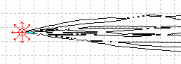
Point sources are represented in WindTrax by any of the icons shown above; their different appearances are for convenience only. At present, sources can represent only one gas at a time, and are assumed to have a constant emission rate during the sampling period. When a source is placed on the map, the forward LS model will be generated automatically; its icon will appear in the upper left corner of the map:

While the simulation is running, lines following the trajectories of the particles being released will appear on the map. To use the computer's resources efficiently, only a small fraction (1/100) of the actual trajectories are drawn. To prevent the trajectories from being displayed, select View|Trajectories from the main menu.
Point source output modePlacing point sources
Specifying point source properties
Grouping point sources
Viewing particle trajectories
Point source-concentration sensor interaction
Back to sources
Point source output mode
Like sensors, sources of tracer gas in WindTrax can be in either known (given) or unknown (find) modes, depending on whether the emission rate is known or sought after by the user. This can be specified at design time by clicking the Measured/Unknown buttons which appear beneath the main tool panel when the Point Source tool is selected; or, once a point source has been placed, its mode can be changed either by selecting it and typing <Ctrl T> to toggle between output modes, or by double-clicking on its icon to display the property editor, and setting its mode on the Measurements tab sheet.
Back to point sourcesPlacing point sources
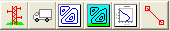
The point source icon is located on the Miscellaneous tool bar:
To add a point source to the map, click on the point source button, move the cursor until its cross-hair is centered over the desired location, and press the mouse button. If more than one point source is to be placed, holding the <Shift> button while clicking the mouse will keep the Point Source tool active; otherwise, the Pointer tool will be retrieved automatically after one source is placed.
By default, point sources are placed in Unknown output mode, at a height of 10 m. The source properties can be modified by double-clicking on either the map icon or the object's name in the Object List form. The default values can be changed by selecting Tools/Environment/Default Values/Point Source from the main menu.
Specifying point source properties
As for all objects in a project, point source properties can be changed by double-clicking either on the source's icon or on its name in the Object List form. Key features include its release height, output mode, and emission rate and/or emission rate units.
If more than one point source is selected when the editor is opened, only those properties that can be modified will be accessible, and any change to a property will affect all selected point sources. For example, because each map object must have a unique name, it is not possible to rename a point source if more than one source is selected. If a particular property differs amongst the selected sources, its data field will remain blank; if the field is modified, the new value will be updated for all selected point sources unless the form is cancelled.
In Version 2, you can select up to 52 emitted different tracers, and can define up to five custom gases. The default is an arbitrary Tracer species, whose molecular weight is equal to that of air for calculations in ppmv and ppbv units.
Back to point sourcesGrouping point sources
A new feature available for WindTrax 1.5 is the abilityto group sets of point sources and have them behave as a single source. The sources can be at different locations and elevations, but are assumed to have the same emission rate. The intention in grouping point sources is to permit a more realistic simulation of sources that look like a distribution of point-like emitters on a relatively small scale (for example, multiple air vents releasing tracer from a building) but still allow a minimum of sensors to estimate their emission rate. (Note that in Version 1.5, no allowance is made for effects of the structure on the mean flow.) The alternative has been to treat barns, etc. as either a single point source or as an area source; it is expected that for measurements taken relatively close by, the distributed point source should be more realistic.
To group a set of point sources, their Group Index must be set to the same non-zero whole value (i.e. 1, 2, 3&). An arbitrary number of groups can be present on the map. To group a large number of sources in a single step, select the entire set and then double-click on any of them; this will open the editor in multiple-edit mode, and allow you to specify the group number and other properties for all selected point sources. To remove one or more sources from a group, set their group indices to zero.
Once grouped, certain properties will be coloured blue in the editor form; this is to alert the user that these properties are common to all sources and modifying them will similarly affect all sources within the group. In particular, emission rate, emission units, and output mode are identical amongst all group members; whereas release height and location are free parameters that can differ between the sources. All members of the group will have the same icon size. You can specify whether or not WindTrax shows the group index on the map; by default, the group index is visible.
Upon completion of a run, grouped sources report both the individual emission rate and the group emission rate. They can be in either unknown or given mode, though all members of the set must have the same mode.
Connecting groups to input and output data files is done by connecting the associated Point Source Group object to the file object as usual. Each grouping of point sources has an automatically-generated Point Source Group object that will appear in the list of connectable objects in the data device editors.
Back to point sourcesViewing particle trajectories
While the simulation is running, lines that follow the trajectories of the particles being released will appear on the map. To use the computer's resources efficiently, only a small fraction (1/100) of the actual trajectories are drawn. To prevent the trajectories from being displayed, select View|Trajectories from the main menu.
Back to point sourcesPoint source-concentration sensor interaction
When the forward LS model runs, it detects events in which the particles being released from a source pass through a volume of space surrounding the spatial locations occupied by concentration sensors present on the map. Each time this occurs, the particle will contribute to the average concentration seen at the given point. A consequence of this approach is that the more detector points present, the more time will be required for the simulation to run.
Although the only physical limitations are the amount of memory in your computer and the number of years you are willing to wait for an answer, it seems prudent to avoid large numbers of concentration detection points. In particular, where contour plots are used, limiting the resolution will keep the simulation from bogging down; for example, a 100 x 100 contour plot grid requires sampling at 10,000 points for each point source present on the map. As the number of sources increases, your result will take longer to generate.
Back to point sourcesProject status
Not all maps that can be drawn represent a valid scenario from which the numerical models can generate meaningful results. For example, if no given-mode anemometers are present, the wind models will be unable to generate a wind field. This will be referred to as the status of a simulation or project. Whenever the map is not valid, the Start and Step buttons and menu items will remain grayed and non-functional.
Status conditionsWorking with project status
Back to User's Guide
Status conditions
In WindTrax, some aspects of a map's design are more significant to the status of a project than others. Status conditions are divided into three categories:
Back to project statusErrors
 Errors are conditions which prevent the simulation from executing, and which are causing the Start button to be grayed. Typical errors include the absence of a required sensor, or an invalid data specification (e.g. sensor height of zero, or wind speed of zero).
Warnings
 Warnings are meant to advise the user of a potentially confusing or unexpected situation; for example, that the backward LS model is using standardized catalogs instead of calculating directly from the map's values. While they will not prevent the model from running, they should be examined.
Notices
 Notices are conditions which are not relevant to the function of the model, but which the user might consider e.g. if the surface roughness is not changed from the default value, a notice will be generated.
Working with project status

Fortunately, WindTrax provides the Project Status object to help the user examine the status of a simulation and, if necessary, correct any errors. It can be accessed at any time by either clicking the Project Status button, located next to the simulation control buttons above the map or by selecting Simulation|Status from the main menu.
Project status formBack to working with status
Project status form
When the status object is activated, a form that lists all the present errors, warnings, and notices present in the project will be displayed. By double clicking with the mouse on a given item on the list, the property editor form for the relevant object will be displayed.
Each item on the list is preceded by a coloured bullet (red () for errors, yellow () for warnings,and green () for notices). Some conditions cannot be corrected by accessing individual objects; for example, if no sensors are present, an error will be generated, but no single object is responsible. In such cases, the bullet will appear darkened ( ,
,  ,
,  ); double clicking on it will have no effect.
Data objects
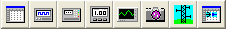
Several objects in WindTrax act as sources and sinks of data during simulations: the Input Data File, Real-time COM Automation Server, Cerex Data File, and Signal Generator provide data to the map from a variety of sources; while the Data Logger, Multi-meter, Chart Recorder, and Camera store or display data generated during an experiment. The tools corresponding to the data objects are located on the Data tool bar:
The following section will describe each of these objects and their uses:
Using data filesInput and output data files
Data cables
The multimeter
The camera
Real-time data COM automation server
Cerex data file
Signal generator
The chart recorder
Back to map objects
Using data files
Although it is possible to run simulations entirely from data provided on the map, most users will wish to provide data from files to simplify the process of analyzing experimental results. In WindTrax, this is accomplished by adding Input File and Output File (or Data Logger) objects to the map. Their icons look like this:


Data from particular columns in these files is connected to properties of individual objects on the map. It is your responsibility to ensure that the columns are correctly specified!
Any parameters that are not connected to an input file column will be taken from the values specified on the map. For example, it is not necessary to provide the height of a sensor as an input file column, since its value will be that of the sensor as it is. If the measurement height varies during the simulation, then you will of course have to associate a column of an input file with the given sensor's height.
Adding an input fileConnecting objects to the input file
Data cables
Working with the data file form
Valid input data
Column delimeters
Missing data flags
Flagged line skipping
Adding output files
Specifying output file columns
Output file options
Copying input file columns to the output file
Back to data objects
Adding an input file
To add an input file to the simulation, click on the Input File button located on the Data tool bar above the map; alternatively, you can select Draw|Data|Input File from the main menu. Once the tool is selected, move the mouse cursor to any point on the map and click the mouse button. The location of the icon isn't important, although other objects might be obscured by the file icon and its data cables (when created).
Double-click on the newly created Input File icon to reveal the properties editor. In WindTrax Version 2, you are required to select the column delimeters separating the file columns. Earlier versions parsed the file and selected them automatically, but there is a wide variety of file formats in use and it was impractical to accommodate them all. Specify the name of the actual data file in the File Name edit box, or click Browse to find its location.
You can inspect the selected file by clicking View, which will open a file viewer. In Version 2, the top lines of the file along with the column header will be displayed on the data form; and the column headers will be displayed on the Connections tab sheet as you move the mouse over them.
Back to Using Data FilesConnecting objects to the input file
Once the file is selected, the File Columns list box on the property editor form will display a column of numbers, each representing one column of the input file. The Available Data tree view to its right will show all objects existing on the map. By clicking on an object's name, its associated properties available for file input will be revealed.
To connect an object property to an input file column, move the mouse cursor until it is over the map object property and press the mouse button down. While holding the button down, drag the mouse over to the left list box. When it is over the number of the column specifying that property, release the button. The two are now connected.
If you wish to remove a connection, using the mouse drag the unwanted data from the left list and drop it anywhere on the right list. Alternatively, the connecting cables can be selected and deleted from the map itself.
To allow more than one object to be connected to a given input file column, hold down the Control key while dropping the property (or clicking the file transfer button).
In WindTrax Version 2, you can also connect file columns to objects by dragging an empty labeled line from the left list box over an available object property in the right list box.
Back to Using Data FilesData cables
To show that a map object's property is connected to a file, a data cable will appear on the map, joining the object to the file:
Because these cables can clutter the map, the user may wish to hide them by selecting View|Data Cables from the main menu. This will toggle the cables between visible and hidden.
Back to data objectsWorking with the data file form
By default, when an object property is dragged over an existing connection in the left list box, the older connection will be replaced. If you wish to associate more than one map object property with a given input file column, hold down the <Control> key while releasing the mouse button. When more than one item is associated with an input column, they will appear listed below "[multiple connections]" in the left box.
To remove a connection using the mouse, simply drag it over the rightlist box and release the mouse button; in this case, the location of release does not matter.
If you have placed properties in the wrong column, they can be rearranged within the left list box by dragging them with the mouse.
Back to Using Data FilesValid input data
It is important that the user ensures that the files contain the correct type of data; for example, a concentration sensor will not readily digest non-numeric data for its concentration value! The only non-numeric data allowed at present is for the specification of stability by either Pasquill-Gifford class (symbols A, B, C, D, E, F, and G) or general class (VU, MU, SU, N, SS, MS, VS).
Back to Using Data FilesColumn delimiters
Five column delimiters are permitted in input and output files: spaces, commas, tabs, colons, and semi-colons. Earlier versions of WindTrax automatically detected which were in use by input files, and parsed the columns accordingly. Due to a number of problems associated with the variety of data file formats in use, Version 2 now requires that you select the column delimeters manually.
For output files, you are free to select from among the five delimiters for the file's format, using the selection box on the data file property editor form.
Back to Using Data FilesMissing data flags
WindTrax must be informed of any missing data symbols present in an input file. By default, it assumes that the sequence -9999 implies that data was absent from the input record, but it can be changed using the property editor. You can choose one of two responses upon encountering this symbol in an input line: WindTrax will either skip over the line or replace the missing data with the last known good value. Some caution must be used; only one symbol is allowed for use at a time. A common problem is to use a similar symbol, such as -999, which would be treated as valid data by WindTrax.
Back to Using Data FilesFlagged line skipping
WindTrax can be forced to ignore (skip over) lines in an input data file by specifying a column that contains "skip line" and "process line" symbols. By default, the symbols are 1 for skip and 0 for process; these can be changed using the input file property editor form. The column is specified by dragging the "Skip line flag" label from the Available Data (right) list box to the appropriate location in the Connections (left) list box. Only one connection is allowed when the flag symbol is specified, so that any existing connections will be removed.
Back to Using Data FilesAdding output files
The procedure for adding output files to a project is much the same as for input files. Select the Output Data File tool and place an output file on the map. Double click it to show its property editor. Specify a name for the output file, or click browse to assist in specifying its directory location; the default location for all output is the directory called Output. Move the mouse cursor over any of the objects listed in the right and click the name to reveal available output data. Use the mouse to drag any of the properties from the right box to the left box, and drop them in the order you want them to appear in the output file; those placed top-most in the list will appear as the left-most columns of the generated output file.
Back to Using Data FilesSpecifying output file columns
In general, more items will be visible than were on the input data file form; this is because some objects have data that can be calculated but not pre-determined (e.g. normalized concentration, from a concentration sensor).
To view the contents of an output file after a simulation has been completed, click on the output file (data logger) icon (before pressing the Rewind button).
Back to Using Data FilesOutput file options
The data file object will generally write a header including all warnings and notices that occurred during the simulation, as well as a key of column identification. This option can be turned off by selecting Tools|Environment from the main menu and clicking the check boxes of the appropriate environment variables. By default, inline messages are written directly within the data as errors and warnings occur while processing input data (for example, when the missing data symbol is encountered in an input file). This feature can be disabled by unchecking the "inline messages" checkbox on the data logger properties editor form.
The user can specify the delimeter character that will be used to separate the data columns; one of five characters is allowed (space, comma, tab, semi-colon, or colon).
Output number format can be specified as either general (a combination of scientific and standard number formats, as appropriate) or scientific. The number of significant figures can be either indeterminate (the default) or fixed.
Back to Using Data FilesCopying input file columns to the output file
It is common for users to copy columns containing date, time, and other information from the input file to the output file. To do this, select the appropriate columns appearing under the Input File object in the Available Data box of the output file's form and drag them to the Column Data box, as you would any other data from the map.
If one or more objects is already connected to a given input file column, hold down the Control key while dropping the output file column (or clicking the file transfer button); otherwise, it will replace the existing connection.
Back to Using Data FilesThe Multimeter

A multimeter is used to display data from objects directly, rather than requiring that they be clicked with the Query Pointer. To add a multimeter measurement to the project, click on the Multimeter button on the Data tool bar above the map or select Draw/Data/Multimeter from the main menu, move the mouse to a suitable location, and then click the map. The multimeter can be connected to any object on the map by double-clicking on the multimeter icon. Both numeric and non-numeric data can be displayed. To disconnect the multimeter, double-click on its icon and click the Disconnect button, or delete the attached data cable.
The multimeter has three display modes: large, small, and label:
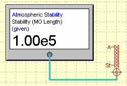
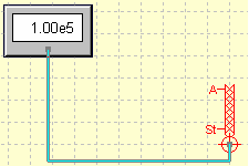
In large mode, both the data and its description are shown; in small mode, only the data is visible; and in label mode, the data label is shown with no rectangular frame.
In all modes, WindTrax 2.0 allows you to enter data directly through the multimeter display provided it is connected to a given, rather than unknown, value. For example, if you connect a multimeter to given-mode surface roughness length Zo, you can click once on its numeric display to reveal an edit box from which you can change Zo directly. This reduces the number of steps; previously, to change Zo you were required to double-click on the map surface to open its property editor, click on the Zo edit box, type its value, and then click on the "Ok" button.
When connected to a non-editable value, multimeters display an off-white background with navy text, and the data value cannot be adjusted.
Back to data objectsThe Camera

The Camera is used to record and display map images during the course of a simulation. At most one camera is permitted on the map. Its tool button is located on the Data tool bar. While the camera is present (and Enabled), it will store images from each step in a simulation in either JPEG or bitmap formats. File names are generated by combining a base file name provided by the user (default is the project name) with a number that is incremented automatically. To specify the file name, increment, output directory, image format, and image compression (for JPEGs), double click on the camera icon. Only the visible portion of the map is stored.
Various identifier stamps can be added to the map images, including the project file name, the time of image creation, and the most recent input line from a user-selectable input data file. The stamps can be located along either the top or bottom edges of the image. These options are specified using the property editor form invoked by double-clicking on the camera icon, or by right-clicking and selecting Properties.
It should be warned that the output image files can be quite large, particularly if they are stored in bitmap format; typically these are on the order of one to two MB. Using JPEG files of reduced quality (typically 50/100) provides a significant reduction in file size (they are on the order of 50 kB).
To view images generated during a simulation, click on the camera icon before pressing the Rewind button. The Viewer form allows the user to step or loop through a multiple set of images. The image files may also be viewed in Edit mode after a simulation has been completed by clicking the View Files button on the Object Editor form.
Back to data objectsThe real-time data COM automation server (Version 1.5)
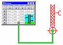
The real-time COM automation server allows WindTrax to receive input data directly from other programs running on the same computer, rather than from a data file. In particular, it provides external programs with a COM-based interface that allows them to control the WindTrax simulation events. The following functions are implemented at present:
- SetChannelCount(long Count) specifies the number of inputs;
- SetChannelName(long Index, BSTR Name) sets the name of a specified input channel;
- SetChannelValue(long Index, BSTR Value) sets the value of the data in the specified channel;
- GetChannelCount(long* Count) returns the number of specified inputs;
- GetChannelName(long Index, BSTR* Name) returns the name associated with a specified channel index;
- GetChannelValue(long Index, BSTR* Value) returns a string version of the data from a specified channel;
- Start() is equivalent to clicking the Run button; it sets WindTrax in Simulation mode if it is in Edit mode;
- Step() starts a simulation step;
- Cancel() aborts the presently executing step, if any;
- Done() causes WindTrax to write data to an output file, if any is present;
- GetCalculationState(long *Result) sets Result to 1 if WindTrax is ready to accept new data or begin a new step, and to 0 otherwise;
- Rewind() returns WindTrax to Edit mode from Done mode.
An example of how to use the real-time COM server is included in the Examples directory. To run the demo, first open project file COM_Demo.wpf in WindTrax. Next, open COM_Demo.xls in Excel. In the Excel file, a simple Visual Basic macro shows the essential programming required to control WindTrax from another program. For further information, please contact me; I may be willing to assist you in integrating WindTrax into your present instrumentation programming.
Back to data objectsThe Cerex data file (Version 2)
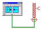
The Cerex Data File object connects WindTrax to data stored by the Cerex sensor system (sonic anemometer + open-path concentration sensor). It automatically determines the tracer species present in the data, adds the required sensors, connects the data inputs and outputsas appropriate, and (when the simulation is running) calculates the model parameters from the sonic data. The user is required only to add and place the source.
Of course, you are still free to connect Cerex files in the same way as standard data files and make the sensor placement and connections manually. The data columns contain tracer concentrations and raw sonic anemometer correlations, which can be connected to a SonicAnemometer sensor. The placement of the data can be observed by looking at the file's column headers.
Back to data objectsThe Signal Generator (Version 2)

WindTrax Version 2 includes the Signal Generator as another data source, which allows you to specify a data signal using an equation. You can include most common mathematical functions (e.g. sine, cosine, tangent, exponential, logarithm, power law, etc.). However, equations are limited to 90 terms. The domain and increment assigned will determine the range and count of the data produced. The object is useful in what-if scenarios - and especially so for debugging the program!
You are free to add as many Signal Generators to the mapas you wish, though it is probably advisable that they be set up to generate the same number of data points in most cases. Once the domain limits have been reached, the generator will stop sending data to the attached objects and the destination value will remain constant.
The Chart Recorder (Version 2)

WindTrax Version 2 introduces the Chart Recorder as another data storage and display option. It is similar to a Data Logger, with two major differences: it displays numeric data from the simulation in chart form as it is generated, and it has a fixed number (15) of output columns. It is another object that was very useful for debugging WindTrax, and provides visual feedback about the progress of the simulation over time. Any number of chart recorders can be added to the map.
Back to data objectsSimulations
In WindTrax, a simulation is the process of generating and examining meteorological results from the designed map. Once a map has been drawn, it is a single button click to run a simulation. The following topics are available:
Simulation ModesControlling a simulation
Ignoring data files
Running in batch mode
Back to User's Guide
Simulation modes
WindTrax simulations can be performed in several ways. If no data files are present, or the Ignore Data Files option is selected, the models will run based on the data specified on the map. If data sources are connected, the simulation can either step through lines in the input file (or signal generator values) one at a time, or run through the entire file.
You can run WindTrax projects in any of four modes:
- immediate mode: the models obtain their boundary conditions from the objects present on the map, and run in a time-independent manner;
- data-driven mode: the models run in time-independent mode, after each line of data is transferred from an input file, signal generator, or the real-time COM server to its associated objects;
- batch mode: all project files listed in a text file, one per line, will be loaded and run sequentially by WindTrax.
- step-wise mode: as in the two modes above, but the user steps through events one at a time.
Any data that is not specifically connected to an input data object will take its value from the model map. For example, if the height of a concentration sensor or the surface roughness length does not change during the simulation, there is no need to specify this in a file; it will remain at the values specified by the user when designing the map.
Back to running simulationsSimulation control
At the top of the map on the main form is a set of buttons used in controlling the progress of a simulation. The same controls can be accessed through the main menu from the Simulation menu item. Five options are available, although not all at the same time:
If none of the buttons is enabled, consult the Project Status by clicking the Status button to the right of the run buttons, or selecting Simulation|Status from the main menu.
Back to running simulationsStarting a simulation

Clicking the Start button or selecting Simulation|Start from the main menu will begin the simulation in either single or batch-run modes (depending on whether any active input data files are present). If no files are present, the simulation will ruin based on data from the map; if files are present and connected to map objects, they will be read and generate new results for each line of data.
If the Start button is not enabled (appears gray) at any time, it implies that there is a problem with the design of the scenario on the map. Click the Status button  appearing at the top of the main form or select Simulation|Status from the main menu.This will display the Project Status form. For more information, see Project Status.
Stepping through a simulation

Clicking the Step button or selecting Simulation|Stepfrom the main menu will cause a single line of the input data file to be read. The simulation will run only to that point and then remain quiescent until the user presses another button. This can be useful for observing the step-by-step progress of the events occurring. If Start is pressed, the model will run in normal mode from the current point to the end of the simulation.
Back to simulation controlsPausing a simulation

Clicking the Pause button or selecting Simulation|Pause from the main menu will temporarily halt the simulation; pressing run or stop will allow it to proceed. While the simulation is halted, WindTrax's use ofsystem resources is reduced to almost none. If it is behaving like a CPU hog and not permitting you to perform other tasks, pausing the simulation may be of benefit. No editing of the project map is permitted while the program is paused, however.
Back to simulation controlsStopping (canceling) a simulation

Occasionally, a simulation may be doing something you hadn't intended it to do. Clicking the Stop button or selecting Simulation|Stop from the main menu will cause the simulation to be cancelled. Any generated data will be lost, since the output files will be erased.
Back to simulation controlsRewinding a simulation

When you have finished examining the results from the simulation, clicking the Rewind button or selecting Simulation|Rewind from the main menu will return WindTrax to its normal editing mode. Until it is pressed, clicking on any object will display its results from the simulation just completed.
Use of the term Rewind may seem obscure; it was chosen because all data files are closed and their file pointers are restored to the start of the file. The next simulation Start will begin exactly as the previous one, unless object parameters or the input files have been changed.
Back to simulation controlsIgnoring data files


When data files are connected to objects on the map,starting the simulation will cause data from the file to be transferred sequentially to the map. However, there are situations in which the user might wish to run What-If scenarios by changing particular values on the map, and run the simulation as if no files were present. To do this, it is possible to temporarily disable all input and output files; either click the Ignore Files button at the top of the map, or select Simulation|Ignore Files from the main menu.
To restore files to an active state, click the Ignore Files button again, or select Simulation|Use Files from the main menu.
Back to running simulationsRunning in batch mode
Running WindTrax in batch mode automates the loading and activation of an arbitrary number of project files. Two steps are required for batch runs: the user must first create and save a plain text file which lists the names of the project files to be run, one per line. The path names must be relative to the directory holding the text file; for example, if text file batch.dat is placed in the main WindTrax directory, and it includes project file name Project1.dat found in directory Projects, the file should include the line ProjectsProject1.dat. Once the text file has been saved, the user invokes batch mode by selecting Simulation | Batch Run& from the main menu, and then specifies the text file containing the project names. It is the responsibility of the user to ensure that each of the listed project files is valid; any that are not will be skipped at batch run time.
Back to running simulationsNumerical models
At present, there are just three models implemented in WindTrax: a simple Monin-Obukhov (analytical) wind model for generating the wind field, and forward and backward Lagrangian stochastic models for predicting tracer gas concentrations and emission rates. The LS models are not created unless required by the sensors and/or sources placed on the map. When a model is created, its icon appears in the upper left corner of the map. If objects requiring the model are deleted, the model will be removed from the simulation and its icon will disappear.
Accessing the modelsThe default wind model
The backward LS mode
The forwards LS model
The LS algebra engine
Unexpected results
Back to User's Guide
Accessing the models
As with all other objects which appear on the map, the properties of the numerical models can be examined and modified by double clicking the mouse over the model's icon on the map. The default location ofthese icons is the upper right corner of the map, although they can be moved. The user can also access the models by selecting Project from the main menu and choosing a model or one of its associated sensors.
Back to numerical modelsThe surface layer model

In present versions, only a Monin-Obukhov similarity theory surface model is implemented in WindTrax. Its functionality has been significantly upgraded in Version 2: it is now responsible for monitoring the wind speed and direction sensors placed on the map and determining how to obtain its parameters (u*, Zo, L, and wind direction angle θ) from them.
There are four options for specifying friction velocity u*:
- it can be entered directly into the model, which is the only option available if no speed sensors are placed on the map.
- the model can derive it from a single given wind speed, along with user-specified Zo and L values.
- the model can calculate it from valid wind speed and temperature profiles. A valid profile requires that at least four wind speeds at different heights are provided; better results are obtained with more measurements and the addition of temperature measurements. See the section on profiles for further information.
- it can be derived from sonic anemometer data.
The surface roughness length Zo can be provided in three ways:
- it can be entered directly on the map surface.
- the model can calculate it from valid wind speed and temperature profiles.
- it can be derived from sonic anemometer data.
Monin-Obukhov length L, which quantifies atmospheric stability, can be specified in several ways:
- it can be entered directly into the model, which is the default option;
- the model can calculate it from a valid Richardson number profile.
- the model can calculate it from valid wind speed and temperature profiles.
- The model can derive it from sonic anemometer data.
The wind direction angle is determined in one of two ways:
- It can be entered directly into the model, if no direction sensors are present.
- It is calculated as the average of measurements from all given-mode direction sensors placed on the map.
By default, WindTrax will assess all sensors placed on the map at any time and select which sources it will use. You can over-ride its selection, though there should not often be a reason to do so. Data sources are chosen based on the following hierarch:
- If a sonic anemometer is present, all parameters will be determined from it. If more than one sonic anemometer is added, all but the first added will be ignored.
- If no sonic anemometer is present but a valid profile of temperature and/or wind speeds is present, all parameters will be calculated from it, although you can opt to specify Zo directly if you wish.
- If no sonic anemometers or profiles are present but a valid Richardson number profile is present, L and u* will be calculated from it; while the surface roughness length Zo will be taken from the map surface.
- If a single cup or standard anemometer is present, u* will be calculated from its data, while L will be taken from the user-specified value and Zo will be obtained from the map surface. This was the only option available in earlier versions of WindTrax.
- If no wind speed sensors are present, all parameters will be obtained from the user-specified values.
Directly specifying atmospheric stability
Directly specifying u* and wind direction
Back to numerical models
Directly specifying surface roughness length Zo
When the default wind model is active, the properties of the surface are assumed to be horizontally uniform in WindTrax. Its roughness can be adjusted either by double clicking anywhere on the background of the map or by selecting Map|Surface from the main menu. The roughness parameter can be either specified directly by the user, if it is known, or estimated by selecting from a descriptive category of surface from the list on the surface properties editor form.
For the default wind model, the roughness length is restricted to 15cm, which implies that WindTrax will not work for surfaces whose canopy is more than about one meter in height. It is important to note that the backward LS model will, by default, convert the specified roughness length to one of its internal categories. This is done to reduce both computation time and the number of touchdown catalogs required. The behaviour can be changed; consult help on the backward LS model.
Directly specifying atmospheric stability
In earlier versions of WindTrax, the atmospheric stability parameter L was determined by the data in a "Stability Sensor". In Version 2, L is accessible directly through the surface layer model's. To modify them while editing the map, double click on the surface layer model's map icon. See the section on Stability Sensor for further information on setting its value manually.
Back to surface layer modelDirectly specifying friction velocity u* and wind direction θ
In WindTrax 2, the friction velocity and wind direction angle are directly accessible through the surface layer model. If you wish to calculate these values yourself and not add any sensors to the map, you can either connect them to an input file or modify them at edit time by double-clicking on the surface layer model's map icon to reveal its property editor.
Back to surface layer modelThe backward LS model
The backward LS model will be created whenever an area source is placed on the map. If no such sources are present, it will not be accessible (since it will not exist). This model has a number of adjustable parameters. To access them, either double-click on the LS model icon appearing in the upper right corner of the map, or select Project|Backward LS Model from the main menu. The following parameters can be adjusted:
Number of particlesVertical tracking
Horizontal tracking
Catalog selection
Zc tolerance
Back to numerical model
Number of particles
Number of Particles on the LS models' property editor forms specifies how many particles will be released by the LS models; its default value is 50,000, although more may be required for a particular situation in order to decrease the models' stochastic error. As might be expected, there is a trade-off between accuracy and time: the larger the number of particles, the longer the model will require to run and/or generate a touchdown catalog with the specified number of particles. The default value was chosen as a balance between the two considerations.
Back to backward LS modelVertical tracking
Vertical tracking identifies the height boundary belowwhich particles may travel without a warning being generated; its default value is 100m. It is an indicator of how well suited the default wind model is to the simulation; if a large number of particles exceeds the upper boundary, it is an indication that the horizontal extent of the simulation probably requires a more sophisticated wind model, to resolve the atmosphere to greater depth than the surface layer alone.
Back to backward LS modelHorizontal tracking
Horizontal tracking specifies the minimumdistance to which particles will be tracked by the model; its default value is 500m. The LS model determines automatically how far particles must be tracked for a given simulation, and will generate a touchdown catalog of the required distance if none exists. The resulting catalog may be of only a very short range, if that was what was required for the situation being simulated. While this is a great advantage for speed of calculation and reducing the size of the generated data file, the catalog will be of limited utility for other simulations due to its (possibly) short range. If "User-defined" is selected, the model will override the minimum range required by thesimulation to produce a catalog of the specified minimum distance.
Which mode the model functions in should be determined by your particular needs. If your work is restricted to short ranges, it may be most efficient to select "Minimum required"; if your simulations willspan a wide range of horizontal scales, it may be better to specify horizontal tracking as the maximum likely range that you will encounter and check "User-defined", to generate a library of reusable catalogs as your work progresses.
Back to backward LS modelCatalog selection
Catalog selection allows the user to choose one of two modes of model operation: in the first, the model will select catalogs based on a predetermined set of sensor heights, roughness lengths, and atmospheric stabilities, where possible. In the second, the model will select or generate touchdowns based on the parameters specified by the map, selecting from previously calculated catalogs if the parameters all lie within the specified ranges. The default is to use standardized values. As with most things, the tradeoff is between accuracy and speed/storage. For the most accurate results, the model should choose values specified by the map (i.e. user); default tolerances are 5% for Zo and 10% for L.
Back to backward LS modelZc tolerance
Zc tolerance determines the maximum percentage difference allowed between a sensor's height (Zs) and a predetermined catalog of touchdowns. For greater accuracy, the value should be smaller; in practice, the default value of 5% is a reasonable compromise.
Back to backward LS modelThe forward LS model
The forward LS model, required for calculations involving point sources, has features similar to those of the Backward LS model. Certain of its parameters can be modified by double-clicking with the mouse on either the model's icon on the map, or on its name in the Object List form.
Back to numerical modelsAlgebra engine

The algebra engine is created automatically whenever an LS model is created. Its function is two-fold: first, it analyzes the simulation for logical consistency in the design of source/concentration sensor relationships; second, when the LS model(s) have finished their calculations, it calculates the final values of emission rate and/or concentration for all unknown values on the map if this is possible.
In order for the algebraic system to be well posed, there must be at least as many known concentrations as unknown emission rates. The converse is not true; given an arbitrary number of known (or calculated) source strengths, an unknown concentration can be calculated at any number of points. For example, a single known concentration value can be used to determine the unknown emission rate Q from an area source; this can then be used to calculate the unknown concentration C at any other point on the map.
If there are more known concentrations than (unknown sources + unknown background), the system of equations is over-determined and thesolution, calculated from Single Value Decomposition (SVD), will be the best least-squares fit to the data provided.
Unexpected resultsBack to numerical models
Unexpected results
The results from an experiment may not be asexpected. At times, negative emission rates or concentrations are predicted; in other cases, a slight change in measured concentration may lead to huge changes in estimated emission rate. Due to the nature of the algebraic system to be solved, the solution may be highly sensitive to uncertainty in the input values. In general, the most robust multi-source systems are those for which the concentration sensors are placed asymmetrically relative to the sources; the greatest sensitivity occurs when the sensors are located very close together.
The sensitivity of a linear system to such changes can bedetermined algebraically from its matrix of coefficients. The Algebra Engine calculates this sensitivity for each simulation run and makes it available for viewing or storage to a file. The property is represented by a number from zero to infinity, with sensitivity being lowest at zero and larger as the number increases. It can be observed by clicking the Query Pointer on the icon for the Algebra Engine, typically located in the upper left corner of the map.
Back to LS Algebra EngineMiscellaneous objects
Location labelText box
Back to User's Guide
Location label

The location label might be useful for annotating project maps; it allows the user to place a marker and text. To add a label, click on the Location Label button on the Miscellaneous Tools button palette or select Draw/Miscellaneous/Location label from the main menu, move the cursor to the desired location, and then click the left mouse button. To change the label text, double click on the marker to reveal the object editor.
Back to miscellaneous objectsText box (Version 1.5)

The text box is another labeling tool for annotating project maps; it allows the user to place one or more lines of text, either within a box or directly onto the background. To add a text box, click on the Text Box button on the Miscellaneous Tools button palette or select Draw/Miscellaneous/Text box from the main menu, move the cursor to the desired location, and then click the left mouse button. To change the text, double click on the text box.
Back to miscellaneous objectsThe Atmosphere object (Version 2)

The Atmosphere object is made visible to the user as an icon (shown above) located in the upper left corner of the map in Version 2. It has many internal responsibilities, primarily related to monitoring the sensors and sources present on the map and managing the models required by them. Its outward significance to the user is that it provides access to the background concentration and a generic "screen temperature" that is used as a default value if no given temperature sensors (thermometer or sonic anemometer) are on the map. You can access these properties in edit mode by double-clicking on the icon.
Back to User's GuideChanges in Version 2.0
Several significant changes have been made to WindTrax in its Version 2 release. A few of these changes might be initially confusing if you are familiar with the earlier versions. Some changes appear trivial and affect only the appearance of the map, while others are not. Here are the most noticeable changes:
- The user interface has undergone one major and several minor changes:
- map tools are now located on tabbed tool bars above the map, instead of along the left side. The increasing number of new tools being added made the older interface more difficult to maintain.
- you can now select individual sensors on a tower using the mouse.
- you can now delete objects by right-clicking on them and selecting Delete.
- input file column headers are now displayed above the file list box in the Input File editor form as the mouse cursor moves over the listed columns.
- buttons have been added above the map to speed access to project file tasks, including loading project files from the history list.
- WindTrax now keeps track of six different input and output directories, instead of defaulting to the Projects, Output, and WindTrax directories.
- The model icons have been shifted to the upper left corner of the map. These icons are actually quite important, and it seemed that they were often being ignored while off in the right corner where they were. They also tended to get lost off the visible edge of the map when project files were transported from one screen resolution to another.
- There is a new icon next to the model icons, representing the Atmosphere object:
The Atmosphere has many internal responsibilities but its outward significance to the user is that it provides access to the background concentration and a generic "screen temperature" that is used as adefault value if no given temperature sensors (thermometer or sonic anemometer) are on the map.
- There is no longer a "Stability Sensor" on the map. If you wish to set the atmosphere's stability directly, it is now accessible through the Surface Layer Model's icon located in the upper left corner of the screen:
- There is no longer a "Background Concentration Sensor" on the map. You can access the background concentration through the Atmosphere icon shown above. Background is a global property and it was rather confusing to have it placed in a localized sensor.
- WindTrax no longer adds a Standard Anemometer to the map at startup, unless requested to do so in the Environment form.
WindTrax can now handle multiple tracers. On the property editor form of all objects that relate to concentration or emission rate, you will find a check list box that allows you to specify the tracer species measured (or emitted). Each species is treated independently, so you can have any combination of source and sensor tracers provided the overall requirement that there be at least one given concentration measurement for each unknown source is satisfied. The background concentration species are updated automatically as sources and sensors are added to the map.
You are free to ignore this new feature, unless your concentrations are measured in ppmv or ppbv. Because molecular weight is required in converting concentrations in ppm or ppb, you will have to select the relevant species for all sensors and sources. By default, an arbitrary tracer is assumed whose molecular weight is equal to that of air.
- WindTrax now accepts a much wider range of data sources for calculating the surface layer model parameters. In earlier versions, u* was primarily determined from a single specified wind speed, while stability and Zo had to be provided by the user. In Version 2, you can:
- provide data directly from a sonic anemometer, from which WindTrax will derive u*, Zo, L, and wind direction;
- provide a profile of wind speeds and temperatures, which WindTrax will use to determine u*, Zo, and L;
- add a two-speed, two-temperature bulk Richardson number profile, which will be used to estimate u* and L;
- provide a single measured wind speed and direction, from which u* will be derived, and specify Zo, and L directly (the default option available in earlier versions.)
- specify all parameters including wind direction directly, without using any sensors.
If more than one of the above sensor data sources is present on the map, WindTrax will select from among them in the order they appear in the above list. For example, if both a profile and a sonic anemometer are present, the profile will be ignored.
- You are now responsible for adding given-mode temperature and pressure sensors to the map if they are required. If no pressure sensors are added, the model will estimate pressure based on the surface elevation, which is now accessible through the Map Surface rather than a pressure sensor. If no temperatures are present, the models will use the default screen temperature associated with the Atmosphere object. By default, elevation is set to 0m ASL and screen temperature to 20C.
- You must now specify a set of column delimeters to be used in parsing input data files. There were too many issues with accommodating all possible data file formats under the auto-detection scheme applied in earlier versions.
- Many new objects have been added: a cup anemometer, which measures only wind speed; a wind vane, which measures direction only; a sonic anemometer, which allows you to interface raw (averaged) sonic anemometer wind statistics correlations; a signal generator, for creating data values from an equation; a chart recorder, for viewing time series of results generated by WindTrax as the simulation proceeds; a transect plot, which allows you to plot data values along an arbitrary line; and a specialized Cerex data file, which automates most of the tasks involved in setting up a project with Cerex systems.
- Project files now end in the extension .wxf rather than .wpf. WindTrax 2 can read projects written with all earlier versions, but older versions can't read Version 2 files. The file storage system was changed to accommodate future expansions in a much more manageable way.
For information on the many other changes introduced with Version 2, go to the About form and click the Changes button.
Back to User's Guide